

200
Practical MATLAB
® Applications for Engineers
Observe that by changing the value of R (R = 3, 9, and 72 Ω), the three solutions for
the second-order differential equation—over, critical, and underdamped—are obtained.
Observe that the analytical solutions completely agree with the MATLAB solutions.
Example 2.30
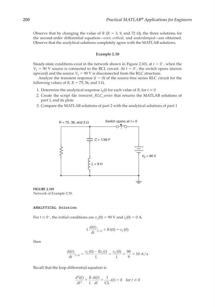
Steady-state conditions exist in the network shown in Figure 2.101, at t = 0
−
, when the
V 0 = 90 V source is connected to the RCL circuit. At t = 0
+
, the switch opens (moves
upward) and the source V 0 = 90 V is disconnected from the RLC structure.
Analyze the transient response (t > 0) of the source-free series RLC circuit for the
following values of R, R = 75, 36, and 3 Ω.
1. Determine the analytical response i R (t) for each value of R, for t ≥ 0
2. Create the script fi le transient_RLC_series that returns the MATLAB solutions of
part 1, and its plots
3. Compare the MATLAB solutions of part 2 with the analytical solutions of part 1
FIGURE 2.101
Network of Example 2.30.
C = 1/36 F
V 0 = 90 V
L = 9 H
R = 75, 36, and 3 Ω
Switch opens at t = 0
ANALYTICAL Solution
For t ≤ 0
−
, the initial conditions are v C (0) = 90 V and i L (0) = 0 A.
L
di t
dt
Ri
v
t
C
( )
( )
( )
ϭ ϩ
ϭ
0
0
0
then
di t
dt
v
R i t
L
v
L
t
C
L
C
( )
( )
( )
( )
/s
ϭ ϭ
ϭ
ϭ
ϭ
0
0
0
9 0
9
10
Ϫ
A
Recall that the loop differential equation is
d i t
dt
R
L
di t
dt
i t
t
2
2
1
0
0
( )
( )
( )
ϩ
ϩ
ϭ
Ն
CL
for
CRC_47760_CH002.indd 200
CRC_47760_CH002.indd 200
7/23/2008 1:39:00 PM
7/23/2008 1:39:00 PM
Practical MATLAB
® Applications for Engineers
Observe that by changing the value of R (R = 3, 9, and 72 Ω), the three solutions for
the second-order differential equation—over, critical, and underdamped—are obtained.
Observe that the analytical solutions completely agree with the MATLAB solutions.
Example 2.30
Steady-state conditions exist in the network shown in Figure 2.101, at t = 0
−
, when the
V 0 = 90 V source is connected to the RCL circuit. At t = 0
+
, the switch opens (moves
upward) and the source V 0 = 90 V is disconnected from the RLC structure.
Analyze the transient response (t > 0) of the source-free series RLC circuit for the
following values of R, R = 75, 36, and 3 Ω.
1. Determine the analytical response i R (t) for each value of R, for t ≥ 0
2. Create the script fi le transient_RLC_series that returns the MATLAB solutions of
part 1, and its plots
3. Compare the MATLAB solutions of part 2 with the analytical solutions of part 1
FIGURE 2.101
Network of Example 2.30.
C = 1/36 F
V 0 = 90 V
L = 9 H
R = 75, 36, and 3 Ω
Switch opens at t = 0
ANALYTICAL Solution
For t ≤ 0
−
, the initial conditions are v C (0) = 90 V and i L (0) = 0 A.
L
di t
dt
Ri
v
t
C
( )
( )
( )
ϭ ϩ
ϭ
0
0
0
then
di t
dt
v
R i t
L
v
L
t
C
L
C
( )
( )
( )
( )
/s
ϭ ϭ
ϭ
ϭ
ϭ
0
0
0
9 0
9
10
Ϫ
A
Recall that the loop differential equation is
d i t
dt
R
L
di t
dt
i t
t
2
2
1
0
0
( )
( )
( )
ϩ
ϩ
ϭ
Ն
CL
for
CRC_47760_CH002.indd 200
CRC_47760_CH002.indd 200
7/23/2008 1:39:00 PM
7/23/2008 1:39:00 PM