

196
Practical MATLAB
® Applications for Engineers
Note that the network shown in Figure 2.95 is an ideal circuit (since there is no resistance, R = 0 in the LC loop for t ≥ 0), and the solution clearly indicates that the current
shows an oscillator behavior with W = 12 rad/s = 1
_____
√
___
LC
and T = π
__
6
s.
Example 2.29
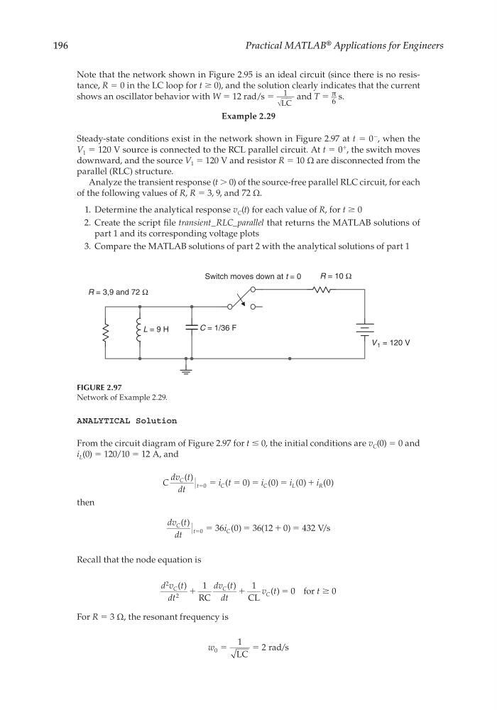
Steady-state conditions exist in the network shown in Figure 2.97 at t = 0
−
, when the
V 1 = 120 V source is connected to the RCL parallel circuit. At t = 0
+
, the switch moves
downward, and the source V 1 = 120 V and resistor R = 10 Ω are disconnected from the
parallel (RLC) structure.
Analyze the transient response (t > 0) of the source-free parallel RLC circuit, for each
of the following values of R, R = 3, 9, and 72 Ω.
1. Determine the analytical response v C (t) for each value of R, for t ≥ 0
2. Create the script fi le transient_RLC_parallel that returns the MATLAB solutions of
part 1 and its corresponding voltage plots
3. Compare the MATLAB solutions of part 2 with the analytical solutions of part 1
FIGURE 2.97
Network of Example 2.29.
L = 9 H
R = 10 Ω
R = 3,9 and 72 Ω
V 1 = 120 V
Switch moves down at t = 0
C = 1/36 F
ANALYTICAL Solution
From the circuit diagram of Figure 2.97 for t ≤ 0, the initial conditions are v C (0) = 0 and
i L (0) = 120/10 = 12 A, and
C
dv t
dt
i t
i
i
i
C
t
C
C
L
R
( )
(
)
( )
( )
( )
ϭ ϭ
ϭ ϭ
ϭ
ϩ
0
0
0
0
0
then
dv t
dt
i
C
t
C
( )
( )
(
)
ϭ ϭ
ϭ
ϩ ϭ
0
36 0
36 12 0
432 V/s
Recall that the node equation is
d v t
dt
dv t
dt
v t
t
C
C
C
2
2
1
1
0
0
( )
( )
( )
ϩ
ϩ
ϭ
Ն
RC
CL
for
For R = 3 Ω, the resonant frequency is
w 0
1
2
ϭ
ϭ
LC
rad/s
CRC_47760_CH002.indd 196
CRC_47760_CH002.indd 196
7/23/2008 1:38:59 PM
7/23/2008 1:38:59 PM
Practical MATLAB
® Applications for Engineers
Note that the network shown in Figure 2.95 is an ideal circuit (since there is no resistance, R = 0 in the LC loop for t ≥ 0), and the solution clearly indicates that the current
shows an oscillator behavior with W = 12 rad/s = 1
_____
√
___
LC
and T = π
__
6
s.
Example 2.29
Steady-state conditions exist in the network shown in Figure 2.97 at t = 0
−
, when the
V 1 = 120 V source is connected to the RCL parallel circuit. At t = 0
+
, the switch moves
downward, and the source V 1 = 120 V and resistor R = 10 Ω are disconnected from the
parallel (RLC) structure.
Analyze the transient response (t > 0) of the source-free parallel RLC circuit, for each
of the following values of R, R = 3, 9, and 72 Ω.
1. Determine the analytical response v C (t) for each value of R, for t ≥ 0
2. Create the script fi le transient_RLC_parallel that returns the MATLAB solutions of
part 1 and its corresponding voltage plots
3. Compare the MATLAB solutions of part 2 with the analytical solutions of part 1
FIGURE 2.97
Network of Example 2.29.
L = 9 H
R = 10 Ω
R = 3,9 and 72 Ω
V 1 = 120 V
Switch moves down at t = 0
C = 1/36 F
ANALYTICAL Solution
From the circuit diagram of Figure 2.97 for t ≤ 0, the initial conditions are v C (0) = 0 and
i L (0) = 120/10 = 12 A, and
C
dv t
dt
i t
i
i
i
C
t
C
C
L
R
( )
(
)
( )
( )
( )
ϭ ϭ
ϭ ϭ
ϭ
ϩ
0
0
0
0
0
then
dv t
dt
i
C
t
C
( )
( )
(
)
ϭ ϭ
ϭ
ϩ ϭ
0
36 0
36 12 0
432 V/s
Recall that the node equation is
d v t
dt
dv t
dt
v t
t
C
C
C
2
2
1
1
0
0
( )
( )
( )
ϩ
ϩ
ϭ
Ն
RC
CL
for
For R = 3 Ω, the resonant frequency is
w 0
1
2
ϭ
ϭ
LC
rad/s
CRC_47760_CH002.indd 196
CRC_47760_CH002.indd 196
7/23/2008 1:38:59 PM
7/23/2008 1:38:59 PM