

8
Practical MATLAB
® Applications for Engineers
The expansion of the function Imp[(t) T ] results in
Imp[( ) ]
(
)
(
)
(
)
() (
)
t
t n T
t nT
t T
t
t T
T
n
ϭ
ϭ
ϩ
ϩ ϩ
ϩ
ϩ ϩ
ϭ
Ϫ
Ϫ
Ϫϱ
ϱ
∑
…
…
( (
)
t nT
Ϫ
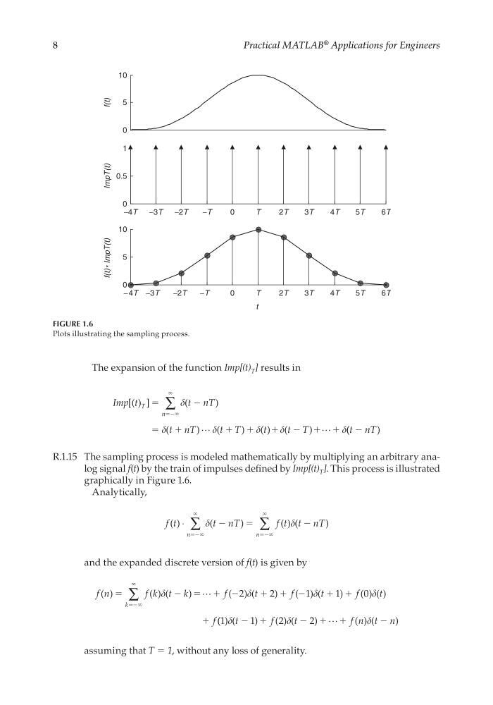
R.1.15 The sampling process is modeled mathematically by multiplying an arbitrary analog signal f(t) by the train of impulses defi ned by Imp[(t) T ]. This process is illustrated
graphically in Figure 1.6.
Analytically,
f t
t nT
f t t nT
n
n
( )
(
)
( ) (
)
⋅
∑
∑
Ϫ
ϭ
ϭ
ϭ
Ϫ
Ϫϱ
ϱ
Ϫϱ
ϱ
and the expanded discrete version of f(t) is given by
f n
f k t k
f
t
f
t
f
t
f
k
( )
( ) (
)
( ) (
)
( ) (
)
( ) ( )
ϭ
ϭ
Ϫ
Ϫ
Ϫϱ
ϱ
Ϫ
ϩ
ϩ ϩ
ϩ ϩ
ϩ
ϭ
∑
2
2
1
1
0
( ( ) (
)
( ) (
)
( ) (
)
1
1
2
2
t
f
t
f n t n
Ϫ
Ϫ
Ϫ
ϩ
ϩ ϩ
assuming that T = 1, without any loss of generality.
0
5
10
f(t)
−4T
−3T
−2T
−T
0
T
2T
3T
4T
5T
6T
0
0.5
1
ImpT(t)
− 4T −3T
−2T
−T
0
T
2T
3T
4T
5T
6T
0
5
10
t
f(t)
* ImpT(t)
FIGURE 1.6
Plots illustrating the sampling process.
CRC_47760_CH001.indd 8
CRC_47760_CH001.indd 8
7/25/2008 4:16:11 PM
7/25/2008 4:16:11 PM
Practical MATLAB
® Applications for Engineers
The expansion of the function Imp[(t) T ] results in
Imp[( ) ]
(
)
(
)
(
)
() (
)
t
t n T
t nT
t T
t
t T
T
n
ϭ
ϭ
ϩ
ϩ ϩ
ϩ
ϩ ϩ
ϭ
Ϫ
Ϫ
Ϫϱ
ϱ
∑
…
…
( (
)
t nT
Ϫ
R.1.15 The sampling process is modeled mathematically by multiplying an arbitrary analog signal f(t) by the train of impulses defi ned by Imp[(t) T ]. This process is illustrated
graphically in Figure 1.6.
Analytically,
f t
t nT
f t t nT
n
n
( )
(
)
( ) (
)
⋅
∑
∑
Ϫ
ϭ
ϭ
ϭ
Ϫ
Ϫϱ
ϱ
Ϫϱ
ϱ
and the expanded discrete version of f(t) is given by
f n
f k t k
f
t
f
t
f
t
f
k
( )
( ) (
)
( ) (
)
( ) (
)
( ) ( )
ϭ
ϭ
Ϫ
Ϫ
Ϫϱ
ϱ
Ϫ
ϩ
ϩ ϩ
ϩ ϩ
ϩ
ϭ
∑
2
2
1
1
0
( ( ) (
)
( ) (
)
( ) (
)
1
1
2
2
t
f
t
f n t n
Ϫ
Ϫ
Ϫ
ϩ
ϩ ϩ
assuming that T = 1, without any loss of generality.
0
5
10
f(t)
−4T
−3T
−2T
−T
0
T
2T
3T
4T
5T
6T
0
0.5
1
ImpT(t)
− 4T −3T
−2T
−T
0
T
2T
3T
4T
5T
6T
0
5
10
t
f(t)
* ImpT(t)
FIGURE 1.6
Plots illustrating the sampling process.
CRC_47760_CH001.indd 8
CRC_47760_CH001.indd 8
7/25/2008 4:16:11 PM
7/25/2008 4:16:11 PM