

178
Practical MATLAB
® Applications for Engineers
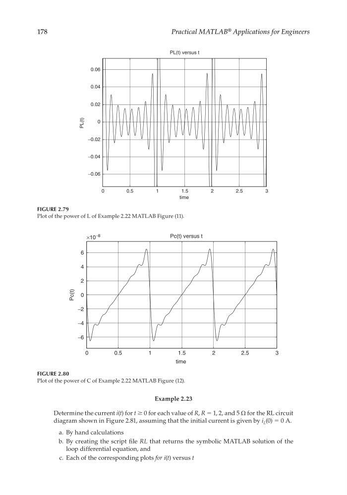
FIGURE 2.79
Plot of the power of L of Example 2.22 MATLAB Figure (11).
0
0.5
1
1.5
2
2.5
3
−0.06
−0.04
−0.02
0
0.02
0.04
0.06
time
PL(t) versus t
PL(t)
FIGURE 2.80
Plot of the power of C of Example 2.22 MATLAB Figure (12).
0
0.5
1
1.5
2
2.5
3
−6
−4
−2
0
2
4
6
×10 −8
time
Pc(t) versus t
Pc(t)
Example 2.23
Determine the current i(t) for t ≥ 0 for each value of R, R = 1, 2, and 5 Ω for the RL circuit
diagram shown in Figure 2.81, assuming that the initial current is given by i L (0) = 0 A.
a. By hand calculations
b. By creating the script fi le RL that returns the symbolic MATLAB solution of the
loop differential equation, and
c. Each of the corresponding plots for i(t) versus t
CRC_47760_CH002.indd 178
CRC_47760_CH002.indd 178
7/23/2008 1:38:55 PM
7/23/2008 1:38:55 PM
Practical MATLAB
® Applications for Engineers
FIGURE 2.79
Plot of the power of L of Example 2.22 MATLAB Figure (11).
0
0.5
1
1.5
2
2.5
3
−0.06
−0.04
−0.02
0
0.02
0.04
0.06
time
PL(t) versus t
PL(t)
FIGURE 2.80
Plot of the power of C of Example 2.22 MATLAB Figure (12).
0
0.5
1
1.5
2
2.5
3
−6
−4
−2
0
2
4
6
×10 −8
time
Pc(t) versus t
Pc(t)
Example 2.23
Determine the current i(t) for t ≥ 0 for each value of R, R = 1, 2, and 5 Ω for the RL circuit
diagram shown in Figure 2.81, assuming that the initial current is given by i L (0) = 0 A.
a. By hand calculations
b. By creating the script fi le RL that returns the symbolic MATLAB solution of the
loop differential equation, and
c. Each of the corresponding plots for i(t) versus t
CRC_47760_CH002.indd 178
CRC_47760_CH002.indd 178
7/23/2008 1:38:55 PM
7/23/2008 1:38:55 PM