

Direct Current and Transient Analysis
173
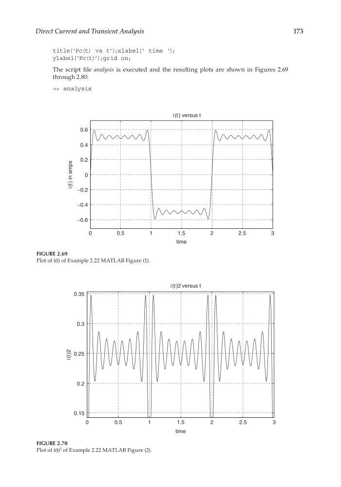
FIGURE 2.69
Plot of i(t) of Example 2.22 MATLAB Figure (1).
0
0.5
1
1.5
2
2.5
3
−0.6
−0.4
−0.2
0
0.2
0.4
0.6
time
i (t ) versus t
i (t ) in amps
FIGURE 2.70
Plot of i(t)
2 of Example 2.22 MATLAB Figure (2).
0
0.5
1
1.5
2
2.5
3
0.15
0.2
0.25
0.3
0.35
time
i(t)2 versus t
i(t)2
title(‘Pc(t) vs t’);xlabel(‘ time ‘);
ylabel(‘Pc(t)’);grid on;
The script fi le analysis is executed and the resulting plots are shown in Figures 2.69
through 2.80.
>> analysis
CRC_47760_CH002.indd 173
CRC_47760_CH002.indd 173
7/23/2008 1:38:54 PM
7/23/2008 1:38:54 PM
173
FIGURE 2.69
Plot of i(t) of Example 2.22 MATLAB Figure (1).
0
0.5
1
1.5
2
2.5
3
−0.6
−0.4
−0.2
0
0.2
0.4
0.6
time
i (t ) versus t
i (t ) in amps
FIGURE 2.70
Plot of i(t)
2 of Example 2.22 MATLAB Figure (2).
0
0.5
1
1.5
2
2.5
3
0.15
0.2
0.25
0.3
0.35
time
i(t)2 versus t
i(t)2
title(‘Pc(t) vs t’);xlabel(‘ time ‘);
ylabel(‘Pc(t)’);grid on;
The script fi le analysis is executed and the resulting plots are shown in Figures 2.69
through 2.80.
>> analysis
CRC_47760_CH002.indd 173
CRC_47760_CH002.indd 173
7/23/2008 1:38:54 PM
7/23/2008 1:38:54 PM