

space, as a natural basis for encoding the geometry of an image local neighborhood
[7, 8]. The subscripted notation will be used to identify partial derivatives with
respect to the coordinates.
The fact that digital images are sampled on a discrete grid may represent some
difficulty as differentiation in the literal sense does not work for discrete signals.
Notably, naive computations are numerically unstable and amplify the highfrequency noise. This difficulty can be overcome by applying the distribution theory, starting from the Leibniz identity for smooth signals [7]:
∇ I ⋆ G
ð
Þ¼ ∇I
ðÞ ⋆ G þ I ⋆∇G
(6)
where ∇ represents the gradient given by its principal components
∇ ¼ ∂=∂x, ∂=∂y
ðÞ . For the whole space if the kernel vanishes fast at infinity, we
have ∇I
ðÞ ⋆ G ¼�I ⋆∇G. Therefore, even for discrete images, by extension, one
can define differentiation in terms of convolution with a differential of a kernel as
∇ G I ≔ � I ⋆∇G
(7)
From this point on, differentiation of a digital image will be interpreted only in
the generalized sense as a convolution with some smooth kernel. In such way,
various local differential geometric invariants can be also incorporated into the
processing. There are several filter families, which possess desirable properties,
which can be exploited for systematic image noise suppression and computation of
differential invariants. These families are formalized by the framework of the scalespace theory. Notable examples are the spatial derivatives of the Gaussian, which
are used in the linear scale-space theory 5.1.
4.1 Differential invariants
There are several types of geometric features, which are useful for segmentation
applications. Typical interesting image features are blobs, filaments, and corners.
Notably, object boundaries can be represented in terms of edges, which can be
approximated by steps in image intensity. All these features can be computed from
the local differential structure of the image. The theory will be exemplified with the
Gaussian derivatives, which, in view of the duality property of Eq. (7), can be used
to compute the image derivatives.
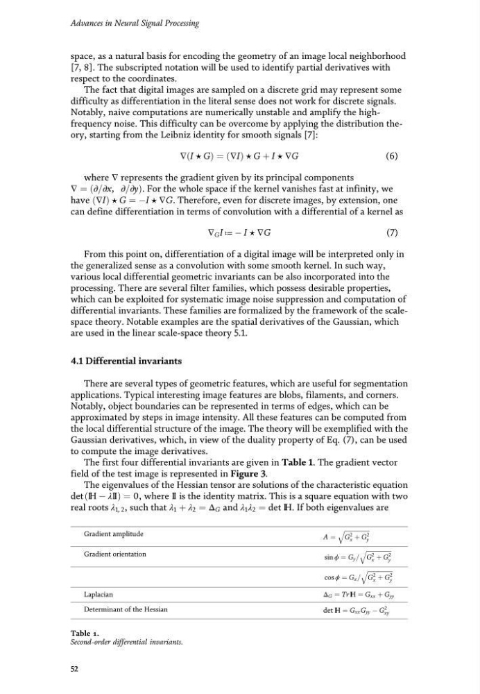
The first four differential invariants are given in Table 1. The gradient vector
field of the test image is represented in Figure 3.
The eigenvalues of the Hessian tensor are solutions of the characteristic equation
det IH � λII
ð
Þ¼0, where II is the identity matrix. This is a square equation with two
real roots λ 1, 2 , such that λ 1 þ λ 2 ¼ Δ G and λ 1 λ 2 ¼ det IH. If both eigenvalues are
Gradient amplitude
A ¼
ffiffiffiffiffiffiffiffiffiffiffiffiffiffiffiffiffi
G
2
x þ G
2
y
q
Gradient orientation
sin ϕ ¼ G y =
ffiffiffiffiffiffiffiffiffiffiffiffiffiffiffiffiffi
G
2
x þ G
2
y
q
cos ϕ ¼ G x =
ffiffiffiffiffiffiffiffiffiffiffiffiffiffiffiffiffi
G
2
x þ G
2
y
q
Laplacian
Δ G ¼ Tr I H ¼ G xx þ G yy
Determinant of the Hessian
det I H ¼ G xx G yy � G
2
xy
Table 1.
Second-order differential invariants.
52
Advances in Neural Signal Processing
[7, 8]. The subscripted notation will be used to identify partial derivatives with
respect to the coordinates.
The fact that digital images are sampled on a discrete grid may represent some
difficulty as differentiation in the literal sense does not work for discrete signals.
Notably, naive computations are numerically unstable and amplify the highfrequency noise. This difficulty can be overcome by applying the distribution theory, starting from the Leibniz identity for smooth signals [7]:
∇ I ⋆ G
ð
Þ¼ ∇I
ðÞ ⋆ G þ I ⋆∇G
(6)
where ∇ represents the gradient given by its principal components
∇ ¼ ∂=∂x, ∂=∂y
ðÞ . For the whole space if the kernel vanishes fast at infinity, we
have ∇I
ðÞ ⋆ G ¼�I ⋆∇G. Therefore, even for discrete images, by extension, one
can define differentiation in terms of convolution with a differential of a kernel as
∇ G I ≔ � I ⋆∇G
(7)
From this point on, differentiation of a digital image will be interpreted only in
the generalized sense as a convolution with some smooth kernel. In such way,
various local differential geometric invariants can be also incorporated into the
processing. There are several filter families, which possess desirable properties,
which can be exploited for systematic image noise suppression and computation of
differential invariants. These families are formalized by the framework of the scalespace theory. Notable examples are the spatial derivatives of the Gaussian, which
are used in the linear scale-space theory 5.1.
4.1 Differential invariants
There are several types of geometric features, which are useful for segmentation
applications. Typical interesting image features are blobs, filaments, and corners.
Notably, object boundaries can be represented in terms of edges, which can be
approximated by steps in image intensity. All these features can be computed from
the local differential structure of the image. The theory will be exemplified with the
Gaussian derivatives, which, in view of the duality property of Eq. (7), can be used
to compute the image derivatives.
The first four differential invariants are given in Table 1. The gradient vector
field of the test image is represented in Figure 3.
The eigenvalues of the Hessian tensor are solutions of the characteristic equation
det IH � λII
ð
Þ¼0, where II is the identity matrix. This is a square equation with two
real roots λ 1, 2 , such that λ 1 þ λ 2 ¼ Δ G and λ 1 λ 2 ¼ det IH. If both eigenvalues are
Gradient amplitude
A ¼
ffiffiffiffiffiffiffiffiffiffiffiffiffiffiffiffiffi
G
2
x þ G
2
y
q
Gradient orientation
sin ϕ ¼ G y =
ffiffiffiffiffiffiffiffiffiffiffiffiffiffiffiffiffi
G
2
x þ G
2
y
q
cos ϕ ¼ G x =
ffiffiffiffiffiffiffiffiffiffiffiffiffiffiffiffiffi
G
2
x þ G
2
y
q
Laplacian
Δ G ¼ Tr I H ¼ G xx þ G yy
Determinant of the Hessian
det I H ¼ G xx G yy � G
2
xy
Table 1.
Second-order differential invariants.
52
Advances in Neural Signal Processing