

124
Network-on-Chip
• m
us
ci : The mapping result taking values {0,1}. The variable is set to 1 if
core c i is mapped onto router u s .
• P
us ut
ci c : The communication path result ∊ {0,1}. The variable is set to 1
if t
j
he communication path exists between routers u s and u t to which
the cores c i and c j have been mapped.
• BW ci cj : The bandwidth requirement between the cores c i and c j
• MD us ut : The Manhattan distance between the routers u s and u t
With this, we proceed to define the constraints for mapping.
1. One-to-one mapping: Each core be mapped to a router and each router
may have at most one core attached to it.
∀u U ∑
us
s ∈ ,
m ci ≤ 1
(5.1)
ci∈C
∀ c
s
i ∈ C, ∑ m
u
ci = 1
(5.2)
us∈U
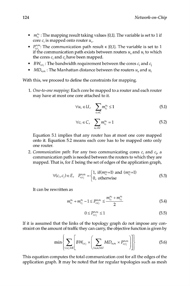
Equation 5.1 implies that any router has at most one core mapped
onto it. Equation 5.2 means each core has to be mapped onto only
one router.
2. Communication path: For any two communicating cores c i and c j , a
communication path is needed between the routers to which they are
mapped. That is, for E being the set of edges of the application graph,
⎧1, if(m us =1) and (m ut =1)
∀(c i , c
P
usut
i
j
j )∈E,
c
c
ci cj = ⎨ ⎨
(5.3)
0,
⎩ otherwise
It can be rewritten as
m
us
+ m
ut
m
us
+ m
ut
− 1 ≤ P
usu
c
t
ci
ci
c j
ci j
≤
j
c
(5.4)
2
0 ≤ P
us ut
ci cj ≤ 1
(5.5)
If it is assumed that the links of the topology graph do not impose any constraint on the amount of traffic they can carry, the objective function is given by
⎧ ∑
⎡
⎛
∑
⎞⎤ ⎫
⎪
⎪
min ⎨
⎢ BW c i cj ×
⎜
MD
s ×
P
usut
u ut
⎟⎥
ci cj
⎬
(5.6)
⎢
⎜
⎟
⎪
⎥
⎩
(ci cj )∈ E E ⎣
⎝
(usut )∈ U
⎠
⎦
⎪ ⎭
This equation computes the total communication cost for all the edges of the
application graph. It may be noted that for regular topologies such as mesh
Network-on-Chip
• m
us
ci : The mapping result taking values {0,1}. The variable is set to 1 if
core c i is mapped onto router u s .
• P
us ut
ci c : The communication path result ∊ {0,1}. The variable is set to 1
if t
j
he communication path exists between routers u s and u t to which
the cores c i and c j have been mapped.
• BW ci cj : The bandwidth requirement between the cores c i and c j
• MD us ut : The Manhattan distance between the routers u s and u t
With this, we proceed to define the constraints for mapping.
1. One-to-one mapping: Each core be mapped to a router and each router
may have at most one core attached to it.
∀u U ∑
us
s ∈ ,
m ci ≤ 1
(5.1)
ci∈C
∀ c
s
i ∈ C, ∑ m
u
ci = 1
(5.2)
us∈U
Equation 5.1 implies that any router has at most one core mapped
onto it. Equation 5.2 means each core has to be mapped onto only
one router.
2. Communication path: For any two communicating cores c i and c j , a
communication path is needed between the routers to which they are
mapped. That is, for E being the set of edges of the application graph,
⎧1, if(m us =1) and (m ut =1)
∀(c i , c
P
usut
i
j
j )∈E,
c
c
ci cj = ⎨ ⎨
(5.3)
0,
⎩ otherwise
It can be rewritten as
m
us
+ m
ut
m
us
+ m
ut
− 1 ≤ P
usu
c
t
ci
ci
c j
ci j
≤
j
c
(5.4)
2
0 ≤ P
us ut
ci cj ≤ 1
(5.5)
If it is assumed that the links of the topology graph do not impose any constraint on the amount of traffic they can carry, the objective function is given by
⎧ ∑
⎡
⎛
∑
⎞⎤ ⎫
⎪
⎪
min ⎨
⎢ BW c i cj ×
⎜
MD
s ×
P
usut
u ut
⎟⎥
ci cj
⎬
(5.6)
⎢
⎜
⎟
⎪
⎥
⎩
(ci cj )∈ E E ⎣
⎝
(usut )∈ U
⎠
⎦
⎪ ⎭
This equation computes the total communication cost for all the edges of the
application graph. It may be noted that for regular topologies such as mesh