

A Model for Electro-osmotic Flow of Pseudoplastic Nanofluids …
197
The coordinates and velocities in the two frames (laboratory and wave frames)
are correlated as follows:
X = x − ct, Y = y, U = u − c and V = v.
(40)
From Eqs. (38–40), we get
Q = F + h 2 − h 1 .
(41)
The time-averaged flow rate (Θ =
1
0
Q(X, t)dt) can be expressed as follows:
Θ = F + 1 + d +
a + b
2
.
(42)
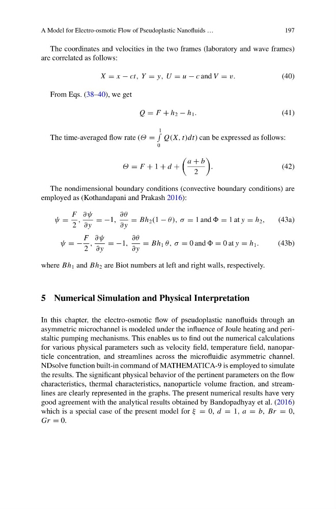
The nondimensional boundary conditions (convective boundary conditions) are
employed as (Kothandapani and Prakash 2016):
ψ =
F
2
,
∂ψ
∂ y
= −1,
∂θ
∂ y
= Bh 2 (1 − θ), σ = 1 and = 1 at y = h 2 ,
(43a)
ψ = −
F
2
,
∂ψ
∂ y
= −1,
∂θ
∂ y
= Bh 1 θ, σ = 0 and = 0 at y = h 1 .
(43b)
where Bh 1 and Bh 2 are Biot numbers at left and right walls, respectively.
5 Numerical Simulation and Physical Interpretation
In this chapter, the electro-osmotic flow of pseudoplastic nanofluids through an
asymmetric microchannel is modeled under the influence of Joule heating and peristaltic pumping mechanisms. This enables us to find out the numerical calculations
for various physical parameters such as velocity field, temperature field, nanoparticle concentration, and streamlines across the microfluidic asymmetric channel.
NDsolve function built-in command of MATHEMATICA-9 is employed to simulate
the results. The significant physical behavior of the pertinent parameters on the flow
characteristics, thermal characteristics, nanoparticle volume fraction, and streamlines are clearly represented in the graphs. The present numerical results have very
good agreement with the analytical results obtained by Bandopadhyay et al. (2016)
which is a special case of the present model for ξ = 0, d = 1, a = b, Br = 0,
Gr = 0.
197
The coordinates and velocities in the two frames (laboratory and wave frames)
are correlated as follows:
X = x − ct, Y = y, U = u − c and V = v.
(40)
From Eqs. (38–40), we get
Q = F + h 2 − h 1 .
(41)
The time-averaged flow rate (Θ =
1
0
Q(X, t)dt) can be expressed as follows:
Θ = F + 1 + d +
a + b
2
.
(42)
The nondimensional boundary conditions (convective boundary conditions) are
employed as (Kothandapani and Prakash 2016):
ψ =
F
2
,
∂ψ
∂ y
= −1,
∂θ
∂ y
= Bh 2 (1 − θ), σ = 1 and = 1 at y = h 2 ,
(43a)
ψ = −
F
2
,
∂ψ
∂ y
= −1,
∂θ
∂ y
= Bh 1 θ, σ = 0 and = 0 at y = h 1 .
(43b)
where Bh 1 and Bh 2 are Biot numbers at left and right walls, respectively.
5 Numerical Simulation and Physical Interpretation
In this chapter, the electro-osmotic flow of pseudoplastic nanofluids through an
asymmetric microchannel is modeled under the influence of Joule heating and peristaltic pumping mechanisms. This enables us to find out the numerical calculations
for various physical parameters such as velocity field, temperature field, nanoparticle concentration, and streamlines across the microfluidic asymmetric channel.
NDsolve function built-in command of MATHEMATICA-9 is employed to simulate
the results. The significant physical behavior of the pertinent parameters on the flow
characteristics, thermal characteristics, nanoparticle volume fraction, and streamlines are clearly represented in the graphs. The present numerical results have very
good agreement with the analytical results obtained by Bandopadhyay et al. (2016)
which is a special case of the present model for ξ = 0, d = 1, a = b, Br = 0,
Gr = 0.