

5.2. Directed edge layered approach
47
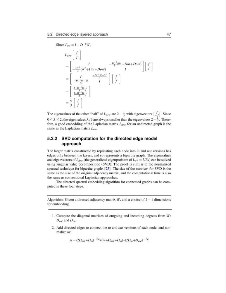
Since L rw = I − D −1 W ,
L drw
f
f
=
I
−
D −1
3 (W +Din+Dout)
−
D −1
3 (W +Din+Dout)
I
f
f
=
I
−D −1 W −2I
3
−D −1 W −2I
3
I
f
f
=
I−D −1 W
3
f
I−D −1 W
3
f
=
λ
3
f
f
The eigenvalues of the other “half” of L drw are 2 −
λ
3 with eigenvectors
f
− f
. Since
0 ≤ λ ≤ 2, the eigenvalues λ /3 are always smaller than the eigenvalues 2−
λ
3 . Therefore, a good embedding of the Laplacian matrix L drw for an undirected graph is the
same as the Laplacian matrix L rw .
5.2.2 SVD computation for the directed edge model
approach
The larger matrix constructed by replicating each node into in and out versions has
edges only between the layers, and so represents a bipartite graph. The eigenvalues
and eigenvectors of L drw (the generalized eigenproblem of L d u = λ Tu) can be solved
using singular value decomposition (SVD). The proof is similar to the normalized
spectral technique for bipartite graphs [23]. The size of the matrices for SVD is the
same as the size of the original adjacency matrix, and the computational time is also
the same as conventional Laplacian approaches.
The directed spectral embedding algorithm for connected graphs can be computed in these four steps.
Algorithm: Given a directed adjacency matrix W , and a choice of k − 1 dimensions
for embedding.
1. Compute the diagonal matrices of outgoing and incoming degrees from W :
D out and D in .
2. Add directed edges to connect the in and out versions of each node, and normalize as:
A = (2D out +D in )
−1/2
∗(W+D out +D in )∗(2D in +D out )
−1/2
.
47
Since L rw = I − D −1 W ,
L drw
f
f
=
I
−
D −1
3 (W +Din+Dout)
−
D −1
3 (W +Din+Dout)
I
f
f
=
I
−D −1 W −2I
3
−D −1 W −2I
3
I
f
f
=
I−D −1 W
3
f
I−D −1 W
3
f
=
λ
3
f
f
The eigenvalues of the other “half” of L drw are 2 −
λ
3 with eigenvectors
f
− f
. Since
0 ≤ λ ≤ 2, the eigenvalues λ /3 are always smaller than the eigenvalues 2−
λ
3 . Therefore, a good embedding of the Laplacian matrix L drw for an undirected graph is the
same as the Laplacian matrix L rw .
5.2.2 SVD computation for the directed edge model
approach
The larger matrix constructed by replicating each node into in and out versions has
edges only between the layers, and so represents a bipartite graph. The eigenvalues
and eigenvectors of L drw (the generalized eigenproblem of L d u = λ Tu) can be solved
using singular value decomposition (SVD). The proof is similar to the normalized
spectral technique for bipartite graphs [23]. The size of the matrices for SVD is the
same as the size of the original adjacency matrix, and the computational time is also
the same as conventional Laplacian approaches.
The directed spectral embedding algorithm for connected graphs can be computed in these four steps.
Algorithm: Given a directed adjacency matrix W , and a choice of k − 1 dimensions
for embedding.
1. Compute the diagonal matrices of outgoing and incoming degrees from W :
D out and D in .
2. Add directed edges to connect the in and out versions of each node, and normalize as:
A = (2D out +D in )
−1/2
∗(W+D out +D in )∗(2D in +D out )
−1/2
.