

5.2. Directed edge layered approach
45
L drw = I − T
−1 M.
An eigendecomposition is used to embed L d or L drw in the standard way.
Computationally, the matrix is now 2n × 2n but, as before, the only new nonzero entries are the diagonal submatrices representing the “vertical” edges. Thus the
matrix is sparse, only one eigendecomposition is required, and so execution times
are much smaller than for the Chung technique.
There are two points corresponding to each node, one corresponding to its
in version and one corresponding to its out version. This has two new, substantial
benefits:
1. The distance between the two versions of a node captures how much asymmetric flow there is through that node. If the flow primarily originates and
terminates in the same subset of other nodes, then this flow will be small.
However, if it originates in one subset of nodes and terminates in another,
this flow will be large (and the distance between versions will also be large).
Thus, this distance in the embedding defines a new, and useful, form of flow
betweenness.
2. Directed edge prediction now becomes possible. For example, if an in version
of one node is embedded close to an out version of another node and they
are not connected in the original graph, then a directed edge from the node
associated with the out-node to the node associated with the in-node can be
predicted.
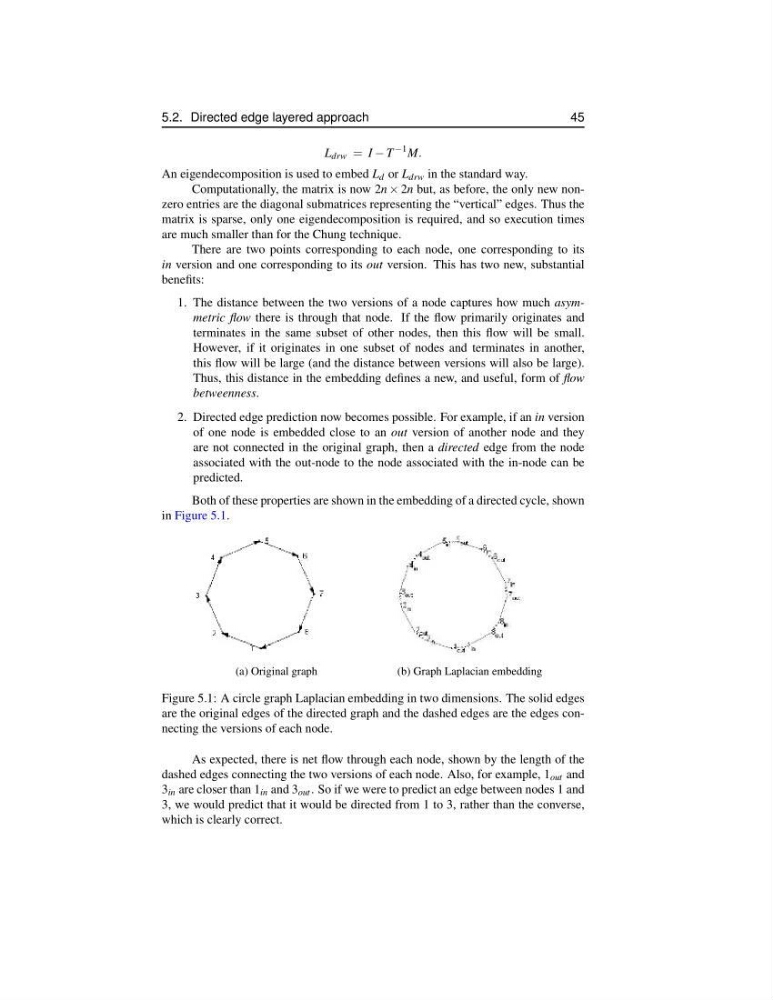
Both of these properties are shown in the embedding of a directed cycle, shown
in Figure 5.1.
(a) Original graph
(b) Graph Laplacian embedding
Figure 5.1: A circle graph Laplacian embedding in two dimensions. The solid edges
are the original edges of the directed graph and the dashed edges are the edges connecting the versions of each node.
As expected, there is net flow through each node, shown by the length of the
dashed edges connecting the two versions of each node. Also, for example, 1 out and
3 in are closer than 1 in and 3 out . So if we were to predict an edge between nodes 1 and
3, we would predict that it would be directed from 1 to 3, rather than the converse,
which is clearly correct.
45
L drw = I − T
−1 M.
An eigendecomposition is used to embed L d or L drw in the standard way.
Computationally, the matrix is now 2n × 2n but, as before, the only new nonzero entries are the diagonal submatrices representing the “vertical” edges. Thus the
matrix is sparse, only one eigendecomposition is required, and so execution times
are much smaller than for the Chung technique.
There are two points corresponding to each node, one corresponding to its
in version and one corresponding to its out version. This has two new, substantial
benefits:
1. The distance between the two versions of a node captures how much asymmetric flow there is through that node. If the flow primarily originates and
terminates in the same subset of other nodes, then this flow will be small.
However, if it originates in one subset of nodes and terminates in another,
this flow will be large (and the distance between versions will also be large).
Thus, this distance in the embedding defines a new, and useful, form of flow
betweenness.
2. Directed edge prediction now becomes possible. For example, if an in version
of one node is embedded close to an out version of another node and they
are not connected in the original graph, then a directed edge from the node
associated with the out-node to the node associated with the in-node can be
predicted.
Both of these properties are shown in the embedding of a directed cycle, shown
in Figure 5.1.
(a) Original graph
(b) Graph Laplacian embedding
Figure 5.1: A circle graph Laplacian embedding in two dimensions. The solid edges
are the original edges of the directed graph and the dashed edges are the edges connecting the versions of each node.
As expected, there is net flow through each node, shown by the length of the
dashed edges connecting the two versions of each node. Also, for example, 1 out and
3 in are closer than 1 in and 3 out . So if we were to predict an edge between nodes 1 and
3, we would predict that it would be directed from 1 to 3, rather than the converse,
which is clearly correct.