

28
Chapter 3. Background
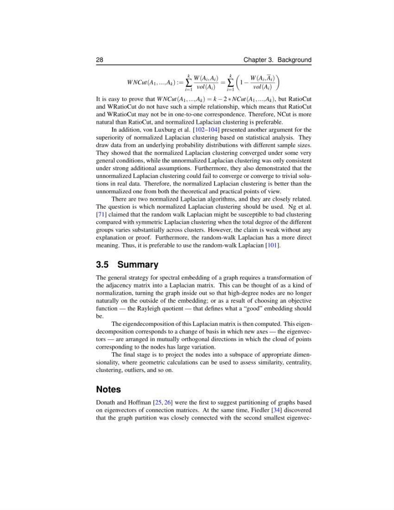
W NCut(A 1 , ..., A k ) :=
k
∑
i=1
W (A i , A i )
vol(A i )
=
k
∑
i=1
1 −
W (A i , A i )
vol(A i )
It is easy to prove that W NCut(A 1 , ..., A k ) = k − 2 ∗ NCut(A 1 , ..., A k ), but RatioCut
and WRatioCut do not have such a simple relationship, which means that RatioCut
and WRatioCut may not be in one-to-one correspondence. Therefore, NCut is more
natural than RatioCut, and normalized Laplacian clustering is preferable.
In addition, von Luxburg et al. [102–104] presented another argument for the
superiority of normalized Laplacian clustering based on statistical analysis. They
draw data from an underlying probability distributions with different sample sizes.
They showed that the normalized Laplacian clustering converged under some very
general conditions, while the unnormalized Laplacian clustering was only consistent
under strong additional assumptions. Furthermore, they also demonstrated that the
unnormalized Laplacian clustering could fail to converge or converge to trivial solutions in real data. Therefore, the normalized Laplacian clustering is better than the
unnormalized one from both the theoretical and practical points of view.
There are two normalized Laplacian algorithms, and they are closely related.
The question is which normalized Laplacian clustering should be used. Ng et al.
[71] claimed that the random walk Laplacian might be susceptible to bad clustering
compared with symmetric Laplacian clustering when the total degree of the different
groups varies substantially across clusters. However, the claim is weak without any
explanation or proof. Furthermore, the random-walk Laplacian has a more direct
meaning. Thus, it is preferable to use the random-walk Laplacian [101].
3.5 Summary
The general strategy for spectral embedding of a graph requires a transformation of
the adjacency matrix into a Laplacian matrix. This can be thought of as a kind of
normalization, turning the graph inside out so that high-degree nodes are no longer
naturally on the outside of the embedding; or as a result of choosing an objective
function — the Rayleigh quotient — that defines what a “good” embedding should
be.
The eigendecomposition of this Laplacian matrix is then computed. This eigendecomposition corresponds to a change of basis in which new axes — the eigenvectors — are arranged in mutually orthogonal directions in which the cloud of points
corresponding to the nodes has large variation.
The final stage is to project the nodes into a subspace of appropriate dimensionality, where geometric calculations can be used to assess similarity, centrality,
clustering, outliers, and so on.
Notes
Donath and Hoffman [25, 26] were the first to suggest partitioning of graphs based
on eigenvectors of connection matrices. At the same time, Fiedler [34] discovered
that the graph partition was closely connected with the second smallest eigenvec-
Chapter 3. Background
W NCut(A 1 , ..., A k ) :=
k
∑
i=1
W (A i , A i )
vol(A i )
=
k
∑
i=1
1 −
W (A i , A i )
vol(A i )
It is easy to prove that W NCut(A 1 , ..., A k ) = k − 2 ∗ NCut(A 1 , ..., A k ), but RatioCut
and WRatioCut do not have such a simple relationship, which means that RatioCut
and WRatioCut may not be in one-to-one correspondence. Therefore, NCut is more
natural than RatioCut, and normalized Laplacian clustering is preferable.
In addition, von Luxburg et al. [102–104] presented another argument for the
superiority of normalized Laplacian clustering based on statistical analysis. They
draw data from an underlying probability distributions with different sample sizes.
They showed that the normalized Laplacian clustering converged under some very
general conditions, while the unnormalized Laplacian clustering was only consistent
under strong additional assumptions. Furthermore, they also demonstrated that the
unnormalized Laplacian clustering could fail to converge or converge to trivial solutions in real data. Therefore, the normalized Laplacian clustering is better than the
unnormalized one from both the theoretical and practical points of view.
There are two normalized Laplacian algorithms, and they are closely related.
The question is which normalized Laplacian clustering should be used. Ng et al.
[71] claimed that the random walk Laplacian might be susceptible to bad clustering
compared with symmetric Laplacian clustering when the total degree of the different
groups varies substantially across clusters. However, the claim is weak without any
explanation or proof. Furthermore, the random-walk Laplacian has a more direct
meaning. Thus, it is preferable to use the random-walk Laplacian [101].
3.5 Summary
The general strategy for spectral embedding of a graph requires a transformation of
the adjacency matrix into a Laplacian matrix. This can be thought of as a kind of
normalization, turning the graph inside out so that high-degree nodes are no longer
naturally on the outside of the embedding; or as a result of choosing an objective
function — the Rayleigh quotient — that defines what a “good” embedding should
be.
The eigendecomposition of this Laplacian matrix is then computed. This eigendecomposition corresponds to a change of basis in which new axes — the eigenvectors — are arranged in mutually orthogonal directions in which the cloud of points
corresponding to the nodes has large variation.
The final stage is to project the nodes into a subspace of appropriate dimensionality, where geometric calculations can be used to assess similarity, centrality,
clustering, outliers, and so on.
Notes
Donath and Hoffman [25, 26] were the first to suggest partitioning of graphs based
on eigenvectors of connection matrices. At the same time, Fiedler [34] discovered
that the graph partition was closely connected with the second smallest eigenvec-