

22
Chapter 3. Background
R L is its Rayleigh quotient [61, 62]. The diagonal of L consists of the degrees of
each of the corresponding nodes, and the off-diagonal entries are the negations of
the weights in the corresponding positions of W . The row sums are all zero, so the
Laplacian can be viewed as a kind of normalization of the cloud of points corresponding to the nodes, since they are now (in a curious way) centered around the
origin.
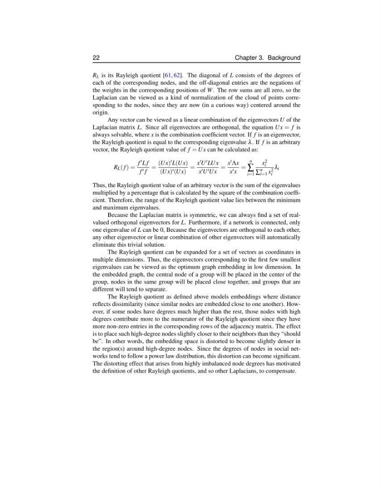
Any vector can be viewed as a linear combination of the eigenvectors U of the
Laplacian matrix L. Since all eigenvectors are orthogonal, the equation Ux = f is
always solvable, where x is the combination coefficient vector. If f is an eigenvector,
the Rayleigh quotient is equal to the corresponding eigenvalue λ . If f is an arbitrary
vector, the Rayleigh quotient value of f = Ux can be calculated as:
R L ( f ) =
f L f
f f
=
(Ux) L(Ux)
(Ux) (Ux)
=
x U LUx
x U Ux
=
x Λx
x x
=
n
∑
i=1
x 2
i
∑
n
i=1 x 2
i
λ i
Thus, the Rayleigh quotient value of an arbitrary vector is the sum of the eigenvalues
multiplied by a percentage that is calculated by the square of the combination coefficient. Therefore, the range of the Rayleigh quotient value lies between the minimum
and maximum eigenvalues.
Because the Laplacian matrix is symmetric, we can always find a set of realvalued orthogonal eigenvectors for L. Furthermore, if a network is connected, only
one eigenvalue of L can be 0, Because the eigenvectors are orthogonal to each other,
any other eigenvector or linear combination of other eigenvectors will automatically
eliminate this trivial solution.
The Rayleigh quotient can be expanded for a set of vectors as coordinates in
multiple dimensions. Thus, the eigenvectors corresponding to the first few smallest
eigenvalues can be viewed as the optimum graph embedding in low dimension. In
the embedded graph, the central node of a group will be placed in the center of the
group, nodes in the same group will be placed close together, and groups that are
different will tend to separate.
The Rayleigh quotient as defined above models embeddings where distance
reflects dissimilarity (since similar nodes are embedded close to one another). However, if some nodes have degrees much higher than the rest, those nodes with high
degrees contribute more to the numerator of the Rayleigh quotient since they have
more non-zero entries in the corresponding rows of the adjacency matrix. The effect
is to place such high-degree nodes slightly closer to their neighbors than they “should
be”. In other words, the embedding space is distorted to become slightly denser in
the region(s) around high-degree nodes. Since the degrees of nodes in social networks tend to follow a power law distribution, this distortion can become significant.
The distorting effect that arises from highly imbalanced node degrees has motivated
the definition of other Rayleigh quotients, and so other Laplacians, to compensate.
Chapter 3. Background
R L is its Rayleigh quotient [61, 62]. The diagonal of L consists of the degrees of
each of the corresponding nodes, and the off-diagonal entries are the negations of
the weights in the corresponding positions of W . The row sums are all zero, so the
Laplacian can be viewed as a kind of normalization of the cloud of points corresponding to the nodes, since they are now (in a curious way) centered around the
origin.
Any vector can be viewed as a linear combination of the eigenvectors U of the
Laplacian matrix L. Since all eigenvectors are orthogonal, the equation Ux = f is
always solvable, where x is the combination coefficient vector. If f is an eigenvector,
the Rayleigh quotient is equal to the corresponding eigenvalue λ . If f is an arbitrary
vector, the Rayleigh quotient value of f = Ux can be calculated as:
R L ( f ) =
f L f
f f
=
(Ux) L(Ux)
(Ux) (Ux)
=
x U LUx
x U Ux
=
x Λx
x x
=
n
∑
i=1
x 2
i
∑
n
i=1 x 2
i
λ i
Thus, the Rayleigh quotient value of an arbitrary vector is the sum of the eigenvalues
multiplied by a percentage that is calculated by the square of the combination coefficient. Therefore, the range of the Rayleigh quotient value lies between the minimum
and maximum eigenvalues.
Because the Laplacian matrix is symmetric, we can always find a set of realvalued orthogonal eigenvectors for L. Furthermore, if a network is connected, only
one eigenvalue of L can be 0, Because the eigenvectors are orthogonal to each other,
any other eigenvector or linear combination of other eigenvectors will automatically
eliminate this trivial solution.
The Rayleigh quotient can be expanded for a set of vectors as coordinates in
multiple dimensions. Thus, the eigenvectors corresponding to the first few smallest
eigenvalues can be viewed as the optimum graph embedding in low dimension. In
the embedded graph, the central node of a group will be placed in the center of the
group, nodes in the same group will be placed close together, and groups that are
different will tend to separate.
The Rayleigh quotient as defined above models embeddings where distance
reflects dissimilarity (since similar nodes are embedded close to one another). However, if some nodes have degrees much higher than the rest, those nodes with high
degrees contribute more to the numerator of the Rayleigh quotient since they have
more non-zero entries in the corresponding rows of the adjacency matrix. The effect
is to place such high-degree nodes slightly closer to their neighbors than they “should
be”. In other words, the embedding space is distorted to become slightly denser in
the region(s) around high-degree nodes. Since the degrees of nodes in social networks tend to follow a power law distribution, this distortion can become significant.
The distorting effect that arises from highly imbalanced node degrees has motivated
the definition of other Rayleigh quotients, and so other Laplacians, to compensate.