193
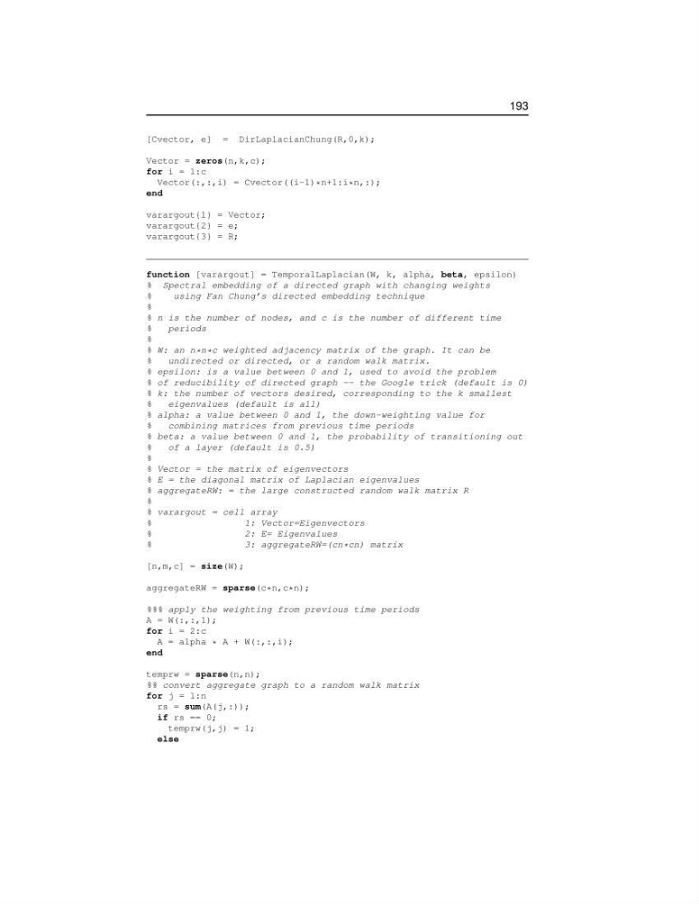
[Cvector, e] = DirLaplacianChung(R,0,k);
Vector = zeros(n,k,c);
for i = 1:c
Vector(:,:,i) = Cvector((i-1) * n+1:i * n,:);
end
varargout{1} = Vector;
varargout{2} = e;
varargout{3} = R;
function [varargout] = TemporalLaplacian(W, k, alpha, beta, epsilon)
% Spectral embedding of a directed graph with changing weights
%
using Fan Chung’s directed embedding technique
%
% n is the number of nodes, and c is the number of different time
%
periods
%
% W: an n * n * c weighted adjacency matrix of the graph. It can be
%
undirected or directed, or a random walk matrix.
% epsilon: is a value between 0 and 1, used to avoid the problem
% of reducibility of directed graph -- the Google trick (default is 0)
% k: the number of vectors desired, corresponding to the k smallest
%
eigenvalues (default is all)
% alpha: a value between 0 and 1, the down-weighting value for
%
combining matrices from previous time periods
% beta: a value between 0 and 1, the probability of transitioning out
%
of a layer (default is 0.5)
%
% Vector = the matrix of eigenvectors
% E = the diagonal matrix of Laplacian eigenvalues
% aggregateRW: = the large constructed random walk matrix R
%
% varargout = cell array
%
1: Vector=Eigenvectors
%
2: E= Eigenvalues
%
3: aggregateRW=(cn * cn) matrix
[n,m,c] = size(W);
aggregateRW = sparse(c * n,c * n);
%%% apply the weighting from previous time periods
A = W(:,:,1);
for i = 2:c
A = alpha * A + W(:,:,i);
end
temprw = sparse(n,n);
%% convert aggregate graph to a random walk matrix
for j = 1:n
rs = sum(A(j,:));
if rs == 0;
temprw(j,j) = 1;
else