

134
Chapter 9. Signed graph-based semi-supervised learning
(a) Synthetic
(b) USPS
(c) ISOLET
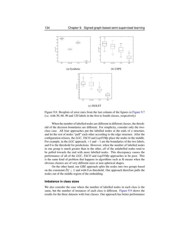
Figure 9.8: Boxplots of error rates from the last column of the figures in Figure 9.7
(i.e. with 30, 60, 90 and 120 labels in the first to fourth classes, respectively)
When the number of labelled nodes are different in different classes, the threshold of the decision boundaries are different. For simplicity, consider only the twoclass case. All four approaches put the labelled nodes at the ends of a structure,
and let the rest of nodes “pull” each other according to the edge structure. After the
configuration relaxes, the LGC, TACO and LapSVMp place the nodes in the middle.
For example, in the LGC approach, +1 and −1 are the boundaries of the two labels,
and 0 is the threshold for predictions. However, when the number of labelled nodes
in one group is much greater than in the other, all of the unlabelled nodes tend to
be pulled towards the end with more labelled nodes. This discrepancy causes the
performance of all of the LGC, TACO and LapSVMp approaches to be poor. This
is the same kind of problem that happens in algorithms such as K-means when the
obvious clusters are of very different sizes or non-spherical shapes.
On the other hand, our GBE approach splits the nodes into two groups based
on the constraint ˆ
D f ⊥ 1 and with 0 as threshold. Our approach therefore pulls the
nodes out of the middle region of the embedding.
Imbalance in class sizes
We also consider the case where the number of labelled nodes in each class is the
same, but the number of instances of each class is different. Figure 9.9 shows the
results for the three datasets with four classes. Our approach has better performance
Chapter 9. Signed graph-based semi-supervised learning
(a) Synthetic
(b) USPS
(c) ISOLET
Figure 9.8: Boxplots of error rates from the last column of the figures in Figure 9.7
(i.e. with 30, 60, 90 and 120 labels in the first to fourth classes, respectively)
When the number of labelled nodes are different in different classes, the threshold of the decision boundaries are different. For simplicity, consider only the twoclass case. All four approaches put the labelled nodes at the ends of a structure,
and let the rest of nodes “pull” each other according to the edge structure. After the
configuration relaxes, the LGC, TACO and LapSVMp place the nodes in the middle.
For example, in the LGC approach, +1 and −1 are the boundaries of the two labels,
and 0 is the threshold for predictions. However, when the number of labelled nodes
in one group is much greater than in the other, all of the unlabelled nodes tend to
be pulled towards the end with more labelled nodes. This discrepancy causes the
performance of all of the LGC, TACO and LapSVMp approaches to be poor. This
is the same kind of problem that happens in algorithms such as K-means when the
obvious clusters are of very different sizes or non-spherical shapes.
On the other hand, our GBE approach splits the nodes into two groups based
on the constraint ˆ
D f ⊥ 1 and with 0 as threshold. Our approach therefore pulls the
nodes out of the middle region of the embedding.
Imbalance in class sizes
We also consider the case where the number of labelled nodes in each class is the
same, but the number of instances of each class is different. Figure 9.9 shows the
results for the three datasets with four classes. Our approach has better performance