

128
Chapter 9. Signed graph-based semi-supervised learning
We also apply our approach to two real-world datasets: the USPS handwritten
digit and the ISOLET Spoken Letter datasets, which are commonly used for graphbased SSL. The ISOLET Spoken Letter dataset [53] was generated by 150 subjects
speaking the name of each English letter of the alphabet twice. Thus there are 300 instances for each letter. We use letters “A” and “B” as a binary classification problem
and letters “A”, “B”, “C”, and “D” as a four-class problem in our experiments.
The USPS data consists of handwritten grayscale 8-bit (16 × 16) images of
digits “0” to “9”. There are 1100 examples of each class, but we only use the first
300 examples of each class to match the size of the ISOLET data. We use digits
“2” and “3” as a binary classification problem and digits “1”, “2”, “3”, and “4” as a
four-class problem.
Both datasets are not graph-based. We convert the data to adjacency matrices
first, and then apply the graph-based SSL. The adjacency matrices are constructed using the K-Nearest Neighbor approach with an RBF kernel, with K set to 5; and the diagonal elements of the created adjacency matrices are set to 0. We add the transpose
to symmetrize the adjacency matrices. The average degree in all the generated adjacency matrices is a little less than 5. The average edge weight is little greater than 0.5.
In all the experiments, we set apw = 150 for the added positive edges, creating
a strong “pull” of labelled nodes towards their class representatives, and anw = 5 for
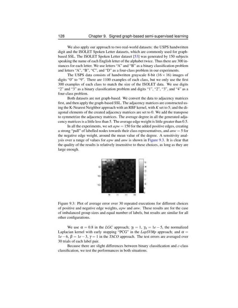
the negative edge weight, around the mean value of the degree. A sensitivity analysis over a range of values for apw and anw is shown in Figure 9.3. It is clear that
the quality of the results is relatively insensitive to these choices, as long as they are
large enough.
Figure 9.3: Plot of average error over 30 repeated executions for different choices
of positive and negative edge weights, apw and anw. These results are for the case
of imbalanced group sizes and equal number of labels, but results are similar for all
other configurations.
We use α = 0.8 in the LGC approach; γ I = 1, γ A = 1e − 5, the normalized
Laplacian kernel with early stopping “PCG” in the LapSVMp approach; and α =
1e − 6, β = 1e − 3, γ = 1 in the TACO approach. The test errors are averaged over
30 trials of each label pair.
Because there are slight differences between binary classification and c-class
classification, we test the performances in both situations.
Chapter 9. Signed graph-based semi-supervised learning
We also apply our approach to two real-world datasets: the USPS handwritten
digit and the ISOLET Spoken Letter datasets, which are commonly used for graphbased SSL. The ISOLET Spoken Letter dataset [53] was generated by 150 subjects
speaking the name of each English letter of the alphabet twice. Thus there are 300 instances for each letter. We use letters “A” and “B” as a binary classification problem
and letters “A”, “B”, “C”, and “D” as a four-class problem in our experiments.
The USPS data consists of handwritten grayscale 8-bit (16 × 16) images of
digits “0” to “9”. There are 1100 examples of each class, but we only use the first
300 examples of each class to match the size of the ISOLET data. We use digits
“2” and “3” as a binary classification problem and digits “1”, “2”, “3”, and “4” as a
four-class problem.
Both datasets are not graph-based. We convert the data to adjacency matrices
first, and then apply the graph-based SSL. The adjacency matrices are constructed using the K-Nearest Neighbor approach with an RBF kernel, with K set to 5; and the diagonal elements of the created adjacency matrices are set to 0. We add the transpose
to symmetrize the adjacency matrices. The average degree in all the generated adjacency matrices is a little less than 5. The average edge weight is little greater than 0.5.
In all the experiments, we set apw = 150 for the added positive edges, creating
a strong “pull” of labelled nodes towards their class representatives, and anw = 5 for
the negative edge weight, around the mean value of the degree. A sensitivity analysis over a range of values for apw and anw is shown in Figure 9.3. It is clear that
the quality of the results is relatively insensitive to these choices, as long as they are
large enough.
Figure 9.3: Plot of average error over 30 repeated executions for different choices
of positive and negative edge weights, apw and anw. These results are for the case
of imbalanced group sizes and equal number of labels, but results are similar for all
other configurations.
We use α = 0.8 in the LGC approach; γ I = 1, γ A = 1e − 5, the normalized
Laplacian kernel with early stopping “PCG” in the LapSVMp approach; and α =
1e − 6, β = 1e − 3, γ = 1 in the TACO approach. The test errors are averaged over
30 trials of each label pair.
Because there are slight differences between binary classification and c-class
classification, we test the performances in both situations.