

126
Chapter 9. Signed graph-based semi-supervised learning
have already discussed, social network graphs are likely to be sparse (although this
algorithm could be applied to graphs generated in other ways, where this might not
be true.)
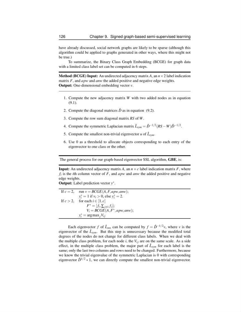
To summarize, the Binary Class Graph Embedding (BCGE) for graph data
with a limited class label set can be computed in 6 steps.
Method (BCGE) Input: An undirected adjacency matrix A, an n×2 label indication
matrix F, and apw and anw the added positive and negative edge weights.
Output: One-dimensional embedding vector v.
1. Compute the new adjacency matrix W with two added nodes as in equation
(9.1).
2. Compute the diagonal matrices ˆ
D as in equation (9.2).
3. Compute the row sum diagonal matrix RS of W .
4. Compute the symmetric Laplacian matrix ˆ
L sym = ˆ
D −1/2 (RS −W ) ˆ
D −1/2 .
5. Compute the smallest non-trivial eigenvector u of ˆ
L sym .
6. Use 0 as a threshold to allocate objects corresponding to each entry of the
eigenvector to one class or the other.
The general process for our graph-based eigenvector SSL algorithm, GBE, is:
Input: An undirected adjacency matrix A, an n × c label indication matrix F, where
f i is the ith column vector of F, and apw and anw the added positive and negative
edge weights.
Output: Label prediction vector y ∗ .
If c = 2, run v = BCGE(A, F, apw, anw);
y ∗
i = 1 if v i > 0, else y ∗
i = 2.
If c > 2, for each i ∈ [1, c]
F ∗ = [ f i , ∑ j =i f j ];
V i = BCGE(A, F ∗ , apw, anw);
y ∗
i = arg max j V i j
Each eigenvector f of ˆ
L sns can be computed by f = ˆ
D −1/2 v, where v is the
eigenvector of the ˆ
L sym . But this step is unnecessary because the modified total
degrees of the nodes do not change for different class labels. When we deal with
the multiple class problem, for each node i, the V i j are on the same scale. As a side
effect, in the multiple class problem, the major part of ˆ
L sym for each label is the
same; only the last two columns and rows need to be changed. Furthermore, because
we know the trivial eigenvalue of the symmetric Laplacian is 0 with corresponding
eigenvector ˆ
D 1/2 ∗ 1, we can directly compute the smallest non-trivial eigenvector.
Chapter 9. Signed graph-based semi-supervised learning
have already discussed, social network graphs are likely to be sparse (although this
algorithm could be applied to graphs generated in other ways, where this might not
be true.)
To summarize, the Binary Class Graph Embedding (BCGE) for graph data
with a limited class label set can be computed in 6 steps.
Method (BCGE) Input: An undirected adjacency matrix A, an n×2 label indication
matrix F, and apw and anw the added positive and negative edge weights.
Output: One-dimensional embedding vector v.
1. Compute the new adjacency matrix W with two added nodes as in equation
(9.1).
2. Compute the diagonal matrices ˆ
D as in equation (9.2).
3. Compute the row sum diagonal matrix RS of W .
4. Compute the symmetric Laplacian matrix ˆ
L sym = ˆ
D −1/2 (RS −W ) ˆ
D −1/2 .
5. Compute the smallest non-trivial eigenvector u of ˆ
L sym .
6. Use 0 as a threshold to allocate objects corresponding to each entry of the
eigenvector to one class or the other.
The general process for our graph-based eigenvector SSL algorithm, GBE, is:
Input: An undirected adjacency matrix A, an n × c label indication matrix F, where
f i is the ith column vector of F, and apw and anw the added positive and negative
edge weights.
Output: Label prediction vector y ∗ .
If c = 2, run v = BCGE(A, F, apw, anw);
y ∗
i = 1 if v i > 0, else y ∗
i = 2.
If c > 2, for each i ∈ [1, c]
F ∗ = [ f i , ∑ j =i f j ];
V i = BCGE(A, F ∗ , apw, anw);
y ∗
i = arg max j V i j
Each eigenvector f of ˆ
L sns can be computed by f = ˆ
D −1/2 v, where v is the
eigenvector of the ˆ
L sym . But this step is unnecessary because the modified total
degrees of the nodes do not change for different class labels. When we deal with
the multiple class problem, for each node i, the V i j are on the same scale. As a side
effect, in the multiple class problem, the major part of ˆ
L sym for each label is the
same; only the last two columns and rows need to be changed. Furthermore, because
we know the trivial eigenvalue of the symmetric Laplacian is 0 with corresponding
eigenvector ˆ
D 1/2 ∗ 1, we can directly compute the smallest non-trivial eigenvector.