

7.2. Applications of temporal networks
89
Period
1
2
3
4
5
6
7
8
9
10
11
Pairs
26
35
68
64
49
68
58
73
60
66
71
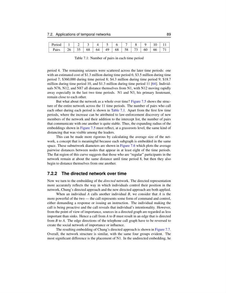
Table 7.1: Number of pairs in each time period
period 4. The remaining seizures were scattered across the later time periods: one
with an estimated cost of $1.3 million during time period 6; $3.5 million during time
period 7; $360,000 during time period 8; $4.3 million during time period 9; $18.7
million during time period 10, and $1.3 million during time period 11 [64]. Individuals N76, N12, and N87 all distance themselves from N1, with N12 moving rapidly
away especially in the last two time periods. N1 and N3, his primary lieutenant,
remain close to each other.
But what about the network as a whole over time? Figure 7.5 shows the structure of the entire network across the 11 time periods. The number of pairs who call
each other during each period is shown in Table 7.1. Apart from the first few time
periods, where the increase can be attributed to law-enforcement discovery of new
members of the network and their addition to the intercept list, the number of pairs
that communicate with one another is quite stable. Thus, the expanding radius of the
embeddings shown in Figure 7.5 must reflect, at a grassroots level, the same kind of
distancing that was visible among the leaders.
This can be made more rigorous by calculating the average size of the network, a concept that is meaningful because each subgraph is embedded in the same
space. These subnetwork diameters are shown in Figure 7.6 which plots the average
pairwise distances between nodes that appear in at least eight of the time periods.
The flat region of this curve suggests that those who are “regular” participants in the
network remain at about the same distance until time period 8, but then they also
begin to distance themselves from one another.
7.2.2 The directed network over time
Now we turn to the embedding of the directed network. The directed representation
more accurately reflects the way in which individuals control their position in the
network, Chung’s directed approach and the new directed approach are both applied.
When an individual A calls another individual B, we consider that A is the
more powerful of the two — the call represents some form of command and control,
either demanding a response or issuing an instruction. The individual making the
call is being proactive and the call reveals that individual’s intentionality. However,
from the point of view of importance, sources in a directed graph are regarded as less
important than sinks. Hence a call from A to B must result in an edge that is directed
from B to A. The edge directions of the telephone call graph have to be reversed to
create the social network of importance or influence.
The resulting embedding of Chung’s directed approach is shown in Figure 7.7.
Overall, the network structure is similar, with the same four groups evident. The
most significant difference is the placement of N1. In the undirected embedding, he
89
Period
1
2
3
4
5
6
7
8
9
10
11
Pairs
26
35
68
64
49
68
58
73
60
66
71
Table 7.1: Number of pairs in each time period
period 4. The remaining seizures were scattered across the later time periods: one
with an estimated cost of $1.3 million during time period 6; $3.5 million during time
period 7; $360,000 during time period 8; $4.3 million during time period 9; $18.7
million during time period 10, and $1.3 million during time period 11 [64]. Individuals N76, N12, and N87 all distance themselves from N1, with N12 moving rapidly
away especially in the last two time periods. N1 and N3, his primary lieutenant,
remain close to each other.
But what about the network as a whole over time? Figure 7.5 shows the structure of the entire network across the 11 time periods. The number of pairs who call
each other during each period is shown in Table 7.1. Apart from the first few time
periods, where the increase can be attributed to law-enforcement discovery of new
members of the network and their addition to the intercept list, the number of pairs
that communicate with one another is quite stable. Thus, the expanding radius of the
embeddings shown in Figure 7.5 must reflect, at a grassroots level, the same kind of
distancing that was visible among the leaders.
This can be made more rigorous by calculating the average size of the network, a concept that is meaningful because each subgraph is embedded in the same
space. These subnetwork diameters are shown in Figure 7.6 which plots the average
pairwise distances between nodes that appear in at least eight of the time periods.
The flat region of this curve suggests that those who are “regular” participants in the
network remain at about the same distance until time period 8, but then they also
begin to distance themselves from one another.
7.2.2 The directed network over time
Now we turn to the embedding of the directed network. The directed representation
more accurately reflects the way in which individuals control their position in the
network, Chung’s directed approach and the new directed approach are both applied.
When an individual A calls another individual B, we consider that A is the
more powerful of the two — the call represents some form of command and control,
either demanding a response or issuing an instruction. The individual making the
call is being proactive and the call reveals that individual’s intentionality. However,
from the point of view of importance, sources in a directed graph are regarded as less
important than sinks. Hence a call from A to B must result in an edge that is directed
from B to A. The edge directions of the telephone call graph have to be reversed to
create the social network of importance or influence.
The resulting embedding of Chung’s directed approach is shown in Figure 7.7.
Overall, the network structure is similar, with the same four groups evident. The
most significant difference is the placement of N1. In the undirected embedding, he