

410
Compact Models for Integrated Circuit Design
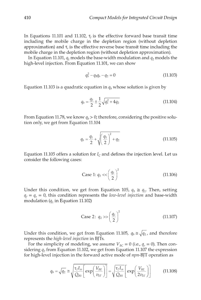
In Equations 11.101 and 11.102, τ f is the effective forward base transit time
including the mobile charge in the depletion region (without depletion
approximation) and τ r is the effective reverse base transit time including the
mobile charge in the depletion region (without depletion approximation).
In Equation 11.101, q 1 models the base-width modulation and q 2 models the
high-level injection. From Equation 11.101, we can show
q q q q
b
b
2
1
2
0
−
− =
(11.103)
Equation 11.103 is a quadratic equation in q b whose solution is given by
q
q
q
q
b = ±
+
1
1
2
2
2
1
2
4
(11.104)
From Equation 11.78, we know q b > 0; therefore, considering the positive solution only, we get from Equation 11.104
q
q
q
q
b = +
+
1
1
2
2
2
2
(11.105)
Equation 11.105 offers a solution for I C and defines the injection level. Let us
consider the following cases:
Case 1: q
q
2
1
2
2
<<
(11.106)
Under this condition, we get from Equation 105, q b ≅ q 1 . Then, setting
q f = q r = 0, this condition represents the low-level injection and base-width
modulation (q 1 in Equation 11.102)
Case 2
2
2
1
2
: q
q
>>
(11.107)
Under this condition, we get from Equation 11.105, q
q
b ≅ 2 , and therefore
represents the high-level injection in BJTs.
For the simplicity of modeling, we assume V BC = 0 (i.e., q r = 0). Then considering q 2 from Equation 11.102, we get from Equation 11.107 the expression
for high-level injection in the forward active mode of npn-BJT operation as
q
q
I
Q
V
v
I
Q
V
v
b
f ss
B
BE
kT
f ss
B
BE
kT
=
≅
=
2
0
0
2
τ
τ
exp
e xp
(11.108)
Compact Models for Integrated Circuit Design
In Equations 11.101 and 11.102, τ f is the effective forward base transit time
including the mobile charge in the depletion region (without depletion
approximation) and τ r is the effective reverse base transit time including the
mobile charge in the depletion region (without depletion approximation).
In Equation 11.101, q 1 models the base-width modulation and q 2 models the
high-level injection. From Equation 11.101, we can show
q q q q
b
b
2
1
2
0
−
− =
(11.103)
Equation 11.103 is a quadratic equation in q b whose solution is given by
q
q
q
q
b = ±
+
1
1
2
2
2
1
2
4
(11.104)
From Equation 11.78, we know q b > 0; therefore, considering the positive solution only, we get from Equation 11.104
q
q
q
q
b = +
+
1
1
2
2
2
2
(11.105)
Equation 11.105 offers a solution for I C and defines the injection level. Let us
consider the following cases:
Case 1: q
q
2
1
2
2
<<
(11.106)
Under this condition, we get from Equation 105, q b ≅ q 1 . Then, setting
q f = q r = 0, this condition represents the low-level injection and base-width
modulation (q 1 in Equation 11.102)
Case 2
2
2
1
2
: q
q
>>
(11.107)
Under this condition, we get from Equation 11.105, q
q
b ≅ 2 , and therefore
represents the high-level injection in BJTs.
For the simplicity of modeling, we assume V BC = 0 (i.e., q r = 0). Then considering q 2 from Equation 11.102, we get from Equation 11.107 the expression
for high-level injection in the forward active mode of npn-BJT operation as
q
q
I
Q
V
v
I
Q
V
v
b
f ss
B
BE
kT
f ss
B
BE
kT
=
≅
=
2
0
0
2
τ
τ
exp
e xp
(11.108)