

194
Mathematical Aspects of Logic Programming Semantics
1 -1
- 1
1
1
1
0.5
A
0.5
B
0.5
C
0.5
0.5
0.5
A
0.5
B
0.5
C
1 -1
-1
1
1
1
1
0.5
A
0.5
B
0.5
C
−0.5
0.5
0.5
0.5
A
0.5
B
0.5
C
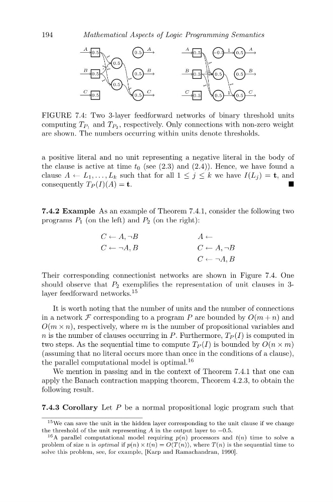
FIGURE 7.4: Two 3-layer feedforward networks of binary threshold units
computing T P1 and T P2 , respectively. Only connections with non-zero weight
are shown. The numbers occurring within units denote thresholds.
a positive literal and no unit representing a negative literal in the body of
the clause is active at time t 0 (see (2.3) and (2.4)). Hence, we have found a
clause A ← L 1 , . . . , L k such that for all 1 ≤ j ≤ k we have I(L j ) = t, and
consequently T P (I)(A) = t.
•
7.4.2 Example As an example of Theorem 7.4.1, consider the following two
programs P 1 (on the left) and P 2 (on the right):
C ← A, ¬B
A ←
C ← ¬A, B
C ← A, ¬B
C ← ¬A, B
Their corresponding connectionist networks are shown in Figure 7.4. One
should observe that P 2 exemplifies the representation of unit clauses in 3layer feedforward networks.
15
It is worth noting that the number of units and the number of connections
in a network F corresponding to a program P are bounded by O(m + n) and
O(m × n), respectively, where m is the number of propositional variables and
n is the number of clauses occurring in P . Furthermore, T P (I) is computed in
two steps. As the sequential time to compute T P (I) is bounded by O(n × m)
(assuming that no literal occurs more than once in the conditions of a clause),
the parallel computational model is optimal.
16
We mention in passing and in the context of Theorem 7.4.1 that one can
apply the Banach contraction mapping theorem, Theorem 4.2.3, to obtain the
following result.
7.4.3 Corollary Let P be a normal propositional logic program such that
15 We can save the unit in the hidden layer corresponding to the unit clause if we change
the threshold of the unit representing A in the output layer to −0.5.
16 A parallel computational model requiring p(n) processors and t(n) time to solve a
problem of size n is optimal if p(n) × t(n) = O(T (n)), where T (n) is the sequential time to
solve this problem, see, for example, [Karp and Ramachandran, 1990].
Mathematical Aspects of Logic Programming Semantics
1 -1
- 1
1
1
1
0.5
A
0.5
B
0.5
C
0.5
0.5
0.5
A
0.5
B
0.5
C
1 -1
-1
1
1
1
1
0.5
A
0.5
B
0.5
C
−0.5
0.5
0.5
0.5
A
0.5
B
0.5
C
FIGURE 7.4: Two 3-layer feedforward networks of binary threshold units
computing T P1 and T P2 , respectively. Only connections with non-zero weight
are shown. The numbers occurring within units denote thresholds.
a positive literal and no unit representing a negative literal in the body of
the clause is active at time t 0 (see (2.3) and (2.4)). Hence, we have found a
clause A ← L 1 , . . . , L k such that for all 1 ≤ j ≤ k we have I(L j ) = t, and
consequently T P (I)(A) = t.
•
7.4.2 Example As an example of Theorem 7.4.1, consider the following two
programs P 1 (on the left) and P 2 (on the right):
C ← A, ¬B
A ←
C ← ¬A, B
C ← A, ¬B
C ← ¬A, B
Their corresponding connectionist networks are shown in Figure 7.4. One
should observe that P 2 exemplifies the representation of unit clauses in 3layer feedforward networks.
15
It is worth noting that the number of units and the number of connections
in a network F corresponding to a program P are bounded by O(m + n) and
O(m × n), respectively, where m is the number of propositional variables and
n is the number of clauses occurring in P . Furthermore, T P (I) is computed in
two steps. As the sequential time to compute T P (I) is bounded by O(n × m)
(assuming that no literal occurs more than once in the conditions of a clause),
the parallel computational model is optimal.
16
We mention in passing and in the context of Theorem 7.4.1 that one can
apply the Banach contraction mapping theorem, Theorem 4.2.3, to obtain the
following result.
7.4.3 Corollary Let P be a normal propositional logic program such that
15 We can save the unit in the hidden layer corresponding to the unit clause if we change
the threshold of the unit representing A in the output layer to −0.5.
16 A parallel computational model requiring p(n) processors and t(n) time to solve a
problem of size n is optimal if p(n) × t(n) = O(T (n)), where T (n) is the sequential time to
solve this problem, see, for example, [Karp and Ramachandran, 1990].