

The arguments in this proof, although correct, are admittedly somewhat
terse, showing only the major steps. We will follow this practice in the rest of the
book, emphasizing the basicideas in a proof and omitting minor details, which
you may want to fill in yourself.
The construction in the previous proof is tedious but important. Let us do
another example to make sure we understand all the steps.
Example 2.13
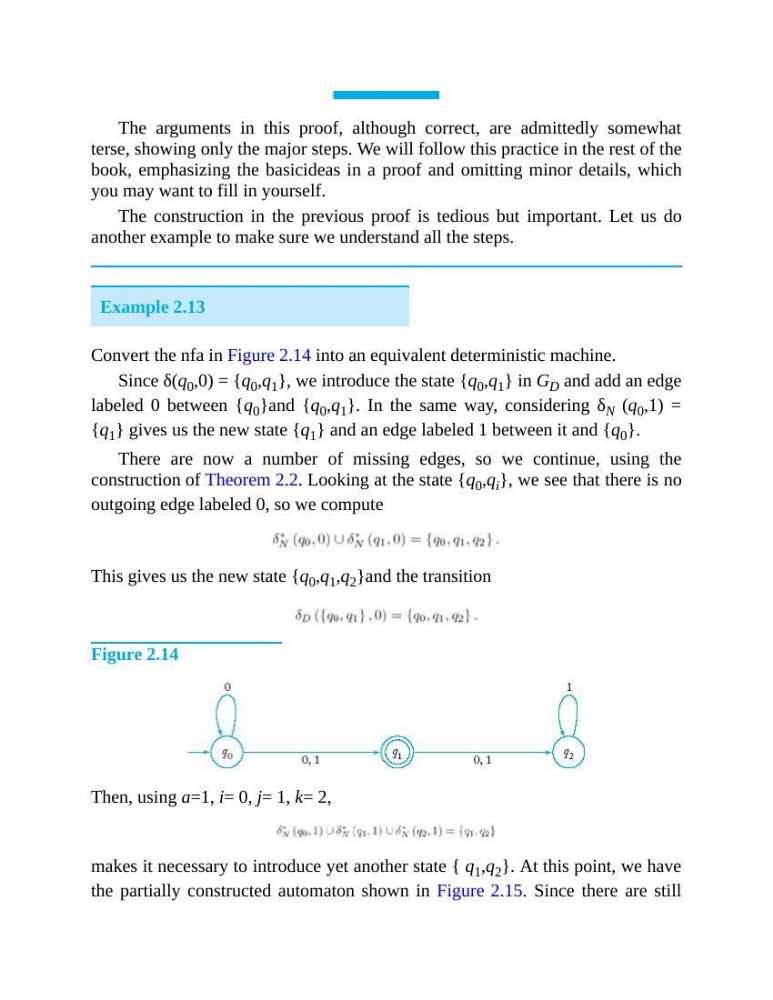
Convert the nfa in Figure 2.14 into an equivalent deterministic machine.
Since δ(q 0 ,0) = {q 0 ,q 1 }, we introduce the state {q 0 ,q 1 } in G D and add an edge
labeled 0 between {q 0 }and {q 0 ,q 1 }. In the same way, considering δ N (q 0 ,1) =
{q 1 } gives us the new state {q 1 } and an edge labeled 1 between it and {q 0 }.
There are now a number of missing edges, so we continue, using the
construction of Theorem 2.2. Looking at the state {q 0 ,q i }, we see that there is no
outgoing edge labeled 0, so we compute
This gives us the new state {q 0 ,q 1 ,q 2 }and the transition
Figure 2.14
Then, using a=1, i= 0, j= 1, k= 2,
makes it necessary to introduce yet another state { q 1 ,q 2 }. At this point, we have
the partially constructed automaton shown in Figure 2.15. Since there are still
terse, showing only the major steps. We will follow this practice in the rest of the
book, emphasizing the basicideas in a proof and omitting minor details, which
you may want to fill in yourself.
The construction in the previous proof is tedious but important. Let us do
another example to make sure we understand all the steps.
Example 2.13
Convert the nfa in Figure 2.14 into an equivalent deterministic machine.
Since δ(q 0 ,0) = {q 0 ,q 1 }, we introduce the state {q 0 ,q 1 } in G D and add an edge
labeled 0 between {q 0 }and {q 0 ,q 1 }. In the same way, considering δ N (q 0 ,1) =
{q 1 } gives us the new state {q 1 } and an edge labeled 1 between it and {q 0 }.
There are now a number of missing edges, so we continue, using the
construction of Theorem 2.2. Looking at the state {q 0 ,q i }, we see that there is no
outgoing edge labeled 0, so we compute
This gives us the new state {q 0 ,q 1 ,q 2 }and the transition
Figure 2.14
Then, using a=1, i= 0, j= 1, k= 2,
makes it necessary to introduce yet another state { q 1 ,q 2 }. At this point, we have
the partially constructed automaton shown in Figure 2.15. Since there are still