

that by construction G M has an edge (q k ,q j ) with label a. Thus, there is a walk in
G M labeled va= w between q i and q j . Since the result is obviously true for n = 1,
we can claim by induction that, for every w ∈ Σ + , implies that there is a walk in
G M from q i to q j labeled w.
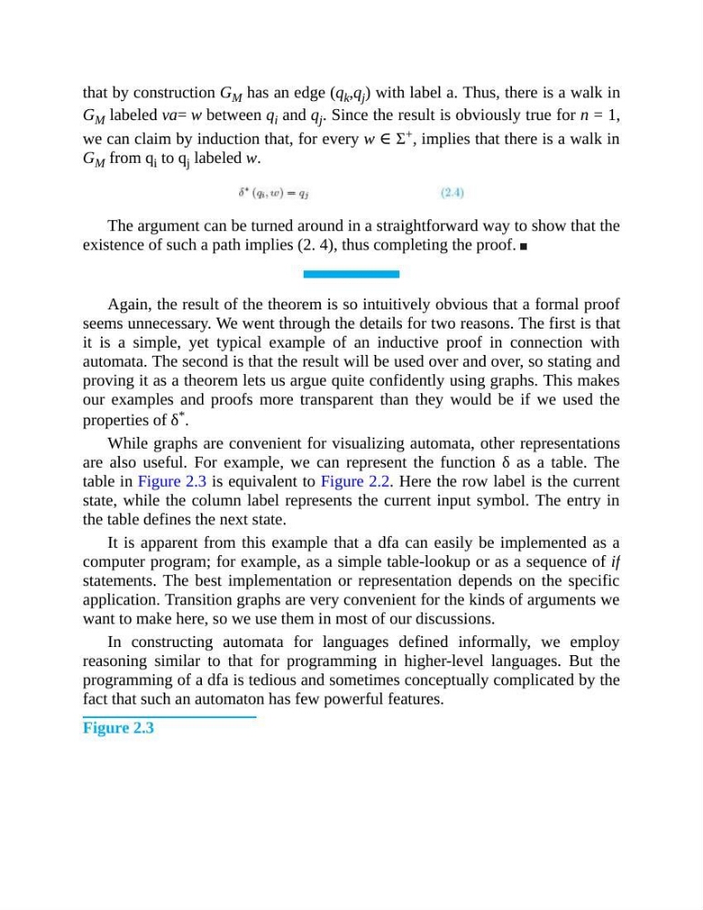
The argument can be turned around in a straightforward way to show that the
existence of such a path implies (2. 4), thus completing the proof.
Again, the result of the theorem is so intuitively obvious that a formal proof
seems unnecessary. We went through the details for two reasons. The first is that
it is a simple, yet typical example of an inductive proof in connection with
automata. The second is that the result will be used over and over, so stating and
proving it as a theorem lets us argue quite confidently using graphs. This makes
our examples and proofs more transparent than they would be if we used the
properties of δ * .
While graphs are convenient for visualizing automata, other representations
are also useful. For example, we can represent the function δ as a table. The
table in Figure 2.3 is equivalent to Figure 2.2. Here the row label is the current
state, while the column label represents the current input symbol. The entry in
the table defines the next state.
It is apparent from this example that a dfa can easily be implemented as a
computer program; for example, as a simple table-lookup or as a sequence of if
statements. The best implementation or representation depends on the specific
application. Transition graphs are very convenient for the kinds of arguments we
want to make here, so we use them in most of our discussions.
In constructing automata for languages defined informally, we employ
reasoning similar to that for programming in higher-level languages. But the
programming of a dfa is tedious and sometimes conceptually complicated by the
fact that such an automaton has few powerful features.
Figure 2.3
G M labeled va= w between q i and q j . Since the result is obviously true for n = 1,
we can claim by induction that, for every w ∈ Σ + , implies that there is a walk in
G M from q i to q j labeled w.
The argument can be turned around in a straightforward way to show that the
existence of such a path implies (2. 4), thus completing the proof.
Again, the result of the theorem is so intuitively obvious that a formal proof
seems unnecessary. We went through the details for two reasons. The first is that
it is a simple, yet typical example of an inductive proof in connection with
automata. The second is that the result will be used over and over, so stating and
proving it as a theorem lets us argue quite confidently using graphs. This makes
our examples and proofs more transparent than they would be if we used the
properties of δ * .
While graphs are convenient for visualizing automata, other representations
are also useful. For example, we can represent the function δ as a table. The
table in Figure 2.3 is equivalent to Figure 2.2. Here the row label is the current
state, while the column label represents the current input symbol. The entry in
the table defines the next state.
It is apparent from this example that a dfa can easily be implemented as a
computer program; for example, as a simple table-lookup or as a sequence of if
statements. The best implementation or representation depends on the specific
application. Transition graphs are very convenient for the kinds of arguments we
want to make here, so we use them in most of our discussions.
In constructing automata for languages defined informally, we employ
reasoning similar to that for programming in higher-level languages. But the
programming of a dfa is tedious and sometimes conceptually complicated by the
fact that such an automaton has few powerful features.
Figure 2.3