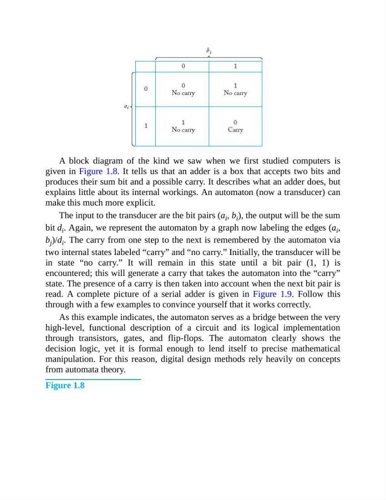
A block diagram of the kind we saw when we first studied computers is
given in Figure 1.8. It tells us that an adder is a box that accepts two bits and
produces their sum bit and a possible carry. It describes what an adder does, but
explains little about its internal workings. An automaton (now a transducer) can
make this much more explicit.
The input to the transducer are the bit pairs (a i , b i ), the output will be the sum
bit d i . Again, we represent the automaton by a graph now labeling the edges (a i ,
b j )/d i . The carry from one step to the next is remembered by the automaton via
two internal states labeled “carry” and “no carry.” Initially, the transducer will be
in state “no carry.” It will remain in this state until a bit pair (1, 1) is
encountered; this will generate a carry that takes the automaton into the “carry”
state. The presence of a carry is then taken into account when the next bit pair is
read. A complete picture of a serial adder is given in Figure 1.9. Follow this
through with a few examples to convince yourself that it works correctly.
As this example indicates, the automaton serves as a bridge between the very
high-level, functional description of a circuit and its logical implementation
through transistors, gates, and flip-flops. The automaton clearly shows the
decision logic, yet it is formal enough to lend itself to precise mathematical
manipulation. For this reason, digital design methods rely heavily on concepts
from automata theory.
Figure 1.8