

δ : Q × ∑ → Q is the transition function,
θ : Q → Γ is the output function,
q 0 ∈ Q is the initial state.
The machine starts in state q 0 , at which time all input is available for
processing. If at time t n the Moore machine is in state q i , the current input
symbol is a, and δ(q j , a) = q j , θ(q j ) = b, the machine will enter state q j and
produce output b.
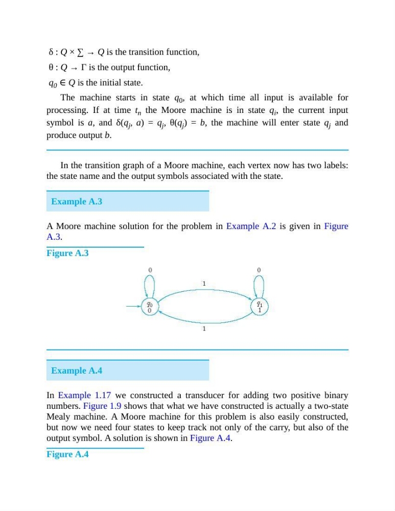
In the transition graph of a Moore machine, each vertex now has two labels:
the state name and the output symbols associated with the state.
Example A.3
A Moore machine solution for the problem in Example A.2 is given in Figure
A.3.
Figure A.3
Example A.4
In Example 1.17 we constructed a transducer for adding two positive binary
numbers. Figure 1.9 shows that what we have constructed is actually a two-state
Mealy machine. A Moore machine for this problem is also easily constructed,
but now we need four states to keep track not only of the carry, but also of the
output symbol. A solution is shown in Figure A.4.
Figure A.4
θ : Q → Γ is the output function,
q 0 ∈ Q is the initial state.
The machine starts in state q 0 , at which time all input is available for
processing. If at time t n the Moore machine is in state q i , the current input
symbol is a, and δ(q j , a) = q j , θ(q j ) = b, the machine will enter state q j and
produce output b.
In the transition graph of a Moore machine, each vertex now has two labels:
the state name and the output symbols associated with the state.
Example A.3
A Moore machine solution for the problem in Example A.2 is given in Figure
A.3.
Figure A.3
Example A.4
In Example 1.17 we constructed a transducer for adding two positive binary
numbers. Figure 1.9 shows that what we have constructed is actually a two-state
Mealy machine. A Moore machine for this problem is also easily constructed,
but now we need four states to keep track not only of the carry, but also of the
output symbol. A solution is shown in Figure A.4.
Figure A.4