

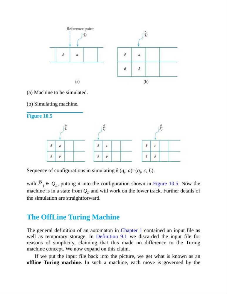
(a) Machine to be simulated.
(b) Simulating machine.
Figure 10.5
Sequence of configurations in simulating δ (q i , a)=(q j , c, L).
with j ∈ Q L , putting it into the configuration shown in Figure 10.5. Now the
machine is in a state from Q L and will work on the lower track. Further details of
the simulation are straightforward.
The OffLine Turing Machine
The general definition of an automaton in Chapter 1 contained an input file as
well as temporary storage. In Definition 9.1 we discarded the input file for
reasons of simplicity, claiming that this made no difference to the Turing
machine concept. We now expand on this claim.
If we put the input file back into the picture, we get what is known as an
offline Turing machine. In such a machine, each move is governed by the
(b) Simulating machine.
Figure 10.5
Sequence of configurations in simulating δ (q i , a)=(q j , c, L).
with j ∈ Q L , putting it into the configuration shown in Figure 10.5. Now the
machine is in a state from Q L and will work on the lower track. Further details of
the simulation are straightforward.
The OffLine Turing Machine
The general definition of an automaton in Chapter 1 contained an input file as
well as temporary storage. In Definition 9.1 we discarded the input file for
reasons of simplicity, claiming that this made no difference to the Turing
machine concept. We now expand on this claim.
If we put the input file back into the picture, we get what is known as an
offline Turing machine. In such a machine, each move is governed by the