

224
S. Okumura et al.
products to focus on the production planning of newly manufactured products. Also,
an inventory holding cost for the collected products h C is omitted to neglect the effect
of the collected product inventory.
16.3.2 Results and Discussion
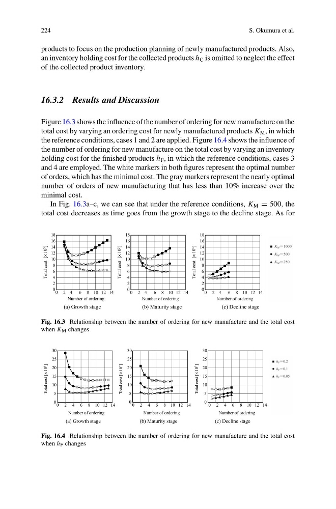
Figure 16.3 shows the influence of the number of ordering for new manufacture on the
total cost by varying an ordering cost for newly manufactured products K M , in which
the reference conditions, cases 1 and 2 are applied. Figure 16.4 shows the influence of
the number of ordering for new manufacture on the total cost by varying an inventory
holding cost for the finished products h F , in which the reference conditions, cases 3
and 4 are employed. The white markers in both figures represent the optimal number
of orders, which has the minimal cost. The gray markers represent the nearly optimal
number of orders of new manufacturing that has less than 10% increase over the
minimal cost.
In Fig. 16.3a–c, we can see that under the reference conditions, K M = 500, the
total cost decreases as time goes from the growth stage to the decline stage. As for
(a) Growth stage
(b) Maturity stage
(c) Decline stage
0
2
4
6
8
10
12
14
16
18
0 2 4
6 8 10 12 14
0 2 4
6 8 10 12 14
0 2 4
6 8 10 12 14
Total cost [ 10 3
]
Number of ordering
0
2
4
6
8
10
12
14
16
18
Total cost [ 10 3
]
Number of ordering
0
2
4
6
8
10
12
14
16
18
Total cost [ 10 3
]
Number of ordering
Fig. 16.3 Relationship between the number of ordering for new manufacture and the total cost
when K M changes
(a) Growth stage
(b) Maturity stage
(c) Decline stage
0
5
10
15
20
25
30
0 2 4 6 8 10 12 14
0 2 4 6 8 10 12 14
0 2 4 6 8 10 12 14
Total cost [ 10 3
]
Number of ordering
0
5
10
15
20
25
30
Total cost [ 10 3
]
Number of ordering
0
5
10
15
20
25
30
Total cost [ 10 3
]
Number of ordering
Fig. 16.4 Relationship between the number of ordering for new manufacture and the total cost
when h F changes
S. Okumura et al.
products to focus on the production planning of newly manufactured products. Also,
an inventory holding cost for the collected products h C is omitted to neglect the effect
of the collected product inventory.
16.3.2 Results and Discussion
Figure 16.3 shows the influence of the number of ordering for new manufacture on the
total cost by varying an ordering cost for newly manufactured products K M , in which
the reference conditions, cases 1 and 2 are applied. Figure 16.4 shows the influence of
the number of ordering for new manufacture on the total cost by varying an inventory
holding cost for the finished products h F , in which the reference conditions, cases 3
and 4 are employed. The white markers in both figures represent the optimal number
of orders, which has the minimal cost. The gray markers represent the nearly optimal
number of orders of new manufacturing that has less than 10% increase over the
minimal cost.
In Fig. 16.3a–c, we can see that under the reference conditions, K M = 500, the
total cost decreases as time goes from the growth stage to the decline stage. As for
(a) Growth stage
(b) Maturity stage
(c) Decline stage
0
2
4
6
8
10
12
14
16
18
0 2 4
6 8 10 12 14
0 2 4
6 8 10 12 14
0 2 4
6 8 10 12 14
Total cost [ 10 3
]
Number of ordering
0
2
4
6
8
10
12
14
16
18
Total cost [ 10 3
]
Number of ordering
0
2
4
6
8
10
12
14
16
18
Total cost [ 10 3
]
Number of ordering
Fig. 16.3 Relationship between the number of ordering for new manufacture and the total cost
when K M changes
(a) Growth stage
(b) Maturity stage
(c) Decline stage
0
5
10
15
20
25
30
0 2 4 6 8 10 12 14
0 2 4 6 8 10 12 14
0 2 4 6 8 10 12 14
Total cost [ 10 3
]
Number of ordering
0
5
10
15
20
25
30
Total cost [ 10 3
]
Number of ordering
0
5
10
15
20
25
30
Total cost [ 10 3
]
Number of ordering
Fig. 16.4 Relationship between the number of ordering for new manufacture and the total cost
when h F changes