

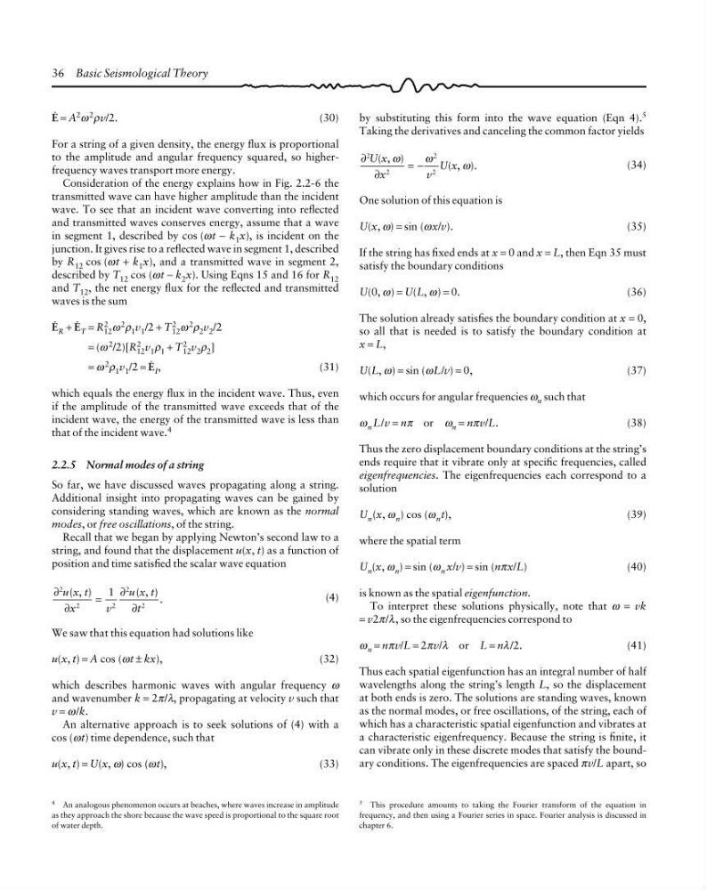
36 Basic Seismological Theory
by substituting this form into the wave equation (Eqn 4). 5
Taking the derivatives and canceling the common factor yields
∂
∂
2
2
2
2
U x
x
v
U x
( , )
( , ).
ω
ω
ω
= −
(34)
One solution of this equation is
U(x, ω) = sin (ωx/v).
(35)
If the string has fixed ends at x = 0 and x = L, then Eqn 35 must
satisfy the boundary conditions
U(0, ω) = U(L, ω) = 0.
(36)
The solution already satisfies the boundary condition at x = 0,
so all that is needed is to satisfy the boundary condition at
x = L,
U(L, ω) = sin (ωL/v) = 0,
(37)
which occurs for angular frequencies ω n such that
ω n L/v = nπ or ω n = nπv/L.
(38)
Thus the zero displacement boundary conditions at the string’s
ends require that it vibrate only at specific frequencies, called
eigenfrequencies. The eigenfrequencies each correspond to a
solution
U n (x, ω n ) cos (ω n t),
(39)
where the spatial term
U n (x, ω n ) = sin (ω n x/v) = sin (nπx/L)
(40)
is known as the spatial eigenfunction.
To interpret these solutions physically, note that ω = vk
= v2π/λ, so the eigenfrequencies correspond to
ω n = nπv/L = 2πv/λ or L = nλ/2.
(41)
Thus each spatial eigenfunction has an integral number of half
wavelengths along the string’s length L, so the displacement
at both ends is zero. The solutions are standing waves, known
as the normal modes, or free oscillations, of the string, each of
which has a characteristic spatial eigenfunction and vibrates at
a characteristic eigenfrequency. Because the string is finite, it
can vibrate only in these discrete modes that satisfy the boundary conditions. The eigenfrequencies are spaced πv/L apart, so
0 = A 2 ω 2 ρv/2.
(30)
For a string of a given density, the energy flux is proportional
to the amplitude and angular frequency squared, so higherfrequency waves transport more energy.
Consideration of the energy explains how in Fig. 2.2-6 the
transmitted wave can have higher amplitude than the incident
wave. To see that an incident wave converting into reflected
and transmitted waves conserves energy, assume that a wave
in segment 1, described by cos (ωt − k 1 x), is incident on the
junction. It gives rise to a reflected wave in segment 1, described
by R 12 cos (ωt + k 1 x), and a transmitted wave in segment 2,
described by T 12 cos (ωt − k 2 x). Using Eqns 15 and 16 for R 12
and T 12 , the net energy flux for the reflected and transmitted
waves is the sum
0 R + 0 T = R 2
12 ω 2 ρ 1 v 1 /2 + T 2
12 ω 2 ρ 2 v 2 /2
= (ω 2 /2)[R 2
12 v 1 ρ 1 + T 2
12 v 2 ρ 2 ]
= ω
2
ρ 1 v 1 /2 = 0 I ,
(31)
which equals the energy flux in the incident wave. Thus, even
if the amplitude of the transmitted wave exceeds that of the
incident wave, the energy of the transmitted wave is less than
that of the incident wave. 4
2.2.5 Normal modes of a string
So far, we have discussed waves propagating along a string.
Additional insight into propagating waves can be gained by
considering standing waves, which are known as the normal
modes, or free oscillations, of the string.
Recall that we began by applying Newton’s second law to a
string, and found that the displacement u(x, t) as a function of
position and time satisfied the scalar wave equation
∂
∂
∂
∂
2
2
2
2
2
1
u x t
x
v
u x t
t
( , )
( , ) .
=
(4)
We saw that this equation had solutions like
u(x, t) = A cos (ωt ± kx),
(32)
which describes harmonic waves with angular frequency ω
and wavenumber k = 2π/λ, propagating at velocity v such that
v = ω /k.
An alternative approach is to seek solutions of (4) with a
cos (ωt) time dependence, such that
u(x, t) = U(x, ω) cos (ωt),
(33)
5 This procedure amounts to taking the Fourier transform of the equation in
frequency, and then using a Fourier series in space. Fourier analysis is discussed in
chapter 6.
4 An analogous phenomenon occurs at beaches, where waves increase in amplitude
as they approach the shore because the wave speed is proportional to the square root
of water depth.
by substituting this form into the wave equation (Eqn 4). 5
Taking the derivatives and canceling the common factor yields
∂
∂
2
2
2
2
U x
x
v
U x
( , )
( , ).
ω
ω
ω
= −
(34)
One solution of this equation is
U(x, ω) = sin (ωx/v).
(35)
If the string has fixed ends at x = 0 and x = L, then Eqn 35 must
satisfy the boundary conditions
U(0, ω) = U(L, ω) = 0.
(36)
The solution already satisfies the boundary condition at x = 0,
so all that is needed is to satisfy the boundary condition at
x = L,
U(L, ω) = sin (ωL/v) = 0,
(37)
which occurs for angular frequencies ω n such that
ω n L/v = nπ or ω n = nπv/L.
(38)
Thus the zero displacement boundary conditions at the string’s
ends require that it vibrate only at specific frequencies, called
eigenfrequencies. The eigenfrequencies each correspond to a
solution
U n (x, ω n ) cos (ω n t),
(39)
where the spatial term
U n (x, ω n ) = sin (ω n x/v) = sin (nπx/L)
(40)
is known as the spatial eigenfunction.
To interpret these solutions physically, note that ω = vk
= v2π/λ, so the eigenfrequencies correspond to
ω n = nπv/L = 2πv/λ or L = nλ/2.
(41)
Thus each spatial eigenfunction has an integral number of half
wavelengths along the string’s length L, so the displacement
at both ends is zero. The solutions are standing waves, known
as the normal modes, or free oscillations, of the string, each of
which has a characteristic spatial eigenfunction and vibrates at
a characteristic eigenfrequency. Because the string is finite, it
can vibrate only in these discrete modes that satisfy the boundary conditions. The eigenfrequencies are spaced πv/L apart, so
0 = A 2 ω 2 ρv/2.
(30)
For a string of a given density, the energy flux is proportional
to the amplitude and angular frequency squared, so higherfrequency waves transport more energy.
Consideration of the energy explains how in Fig. 2.2-6 the
transmitted wave can have higher amplitude than the incident
wave. To see that an incident wave converting into reflected
and transmitted waves conserves energy, assume that a wave
in segment 1, described by cos (ωt − k 1 x), is incident on the
junction. It gives rise to a reflected wave in segment 1, described
by R 12 cos (ωt + k 1 x), and a transmitted wave in segment 2,
described by T 12 cos (ωt − k 2 x). Using Eqns 15 and 16 for R 12
and T 12 , the net energy flux for the reflected and transmitted
waves is the sum
0 R + 0 T = R 2
12 ω 2 ρ 1 v 1 /2 + T 2
12 ω 2 ρ 2 v 2 /2
= (ω 2 /2)[R 2
12 v 1 ρ 1 + T 2
12 v 2 ρ 2 ]
= ω
2
ρ 1 v 1 /2 = 0 I ,
(31)
which equals the energy flux in the incident wave. Thus, even
if the amplitude of the transmitted wave exceeds that of the
incident wave, the energy of the transmitted wave is less than
that of the incident wave. 4
2.2.5 Normal modes of a string
So far, we have discussed waves propagating along a string.
Additional insight into propagating waves can be gained by
considering standing waves, which are known as the normal
modes, or free oscillations, of the string.
Recall that we began by applying Newton’s second law to a
string, and found that the displacement u(x, t) as a function of
position and time satisfied the scalar wave equation
∂
∂
∂
∂
2
2
2
2
2
1
u x t
x
v
u x t
t
( , )
( , ) .
=
(4)
We saw that this equation had solutions like
u(x, t) = A cos (ωt ± kx),
(32)
which describes harmonic waves with angular frequency ω
and wavenumber k = 2π/λ, propagating at velocity v such that
v = ω /k.
An alternative approach is to seek solutions of (4) with a
cos (ωt) time dependence, such that
u(x, t) = U(x, ω) cos (ωt),
(33)
5 This procedure amounts to taking the Fourier transform of the equation in
frequency, and then using a Fourier series in space. Fourier analysis is discussed in
chapter 6.
4 An analogous phenomenon occurs at beaches, where waves increase in amplitude
as they approach the shore because the wave speed is proportional to the square root
of water depth.