

34 Basic Seismological Theory
the middle again (time 8), it gives rise to the small reflection
with amplitude R 12 (−1)R 12 = −0.11 and a transmitted pulse
with amplitude R 12 (−1)T 12 = 0.22.
By time 14, the original pulse that traveled to the right has
been transmitted to segment 2, inverted by reflection off the
right boundary (time 8), and is now incident on the junction
from the right. The reflection and transmission coefficients for
a wave incident from segment 2 are R 21 = 0.33, T 21 = 1.33.
Thus the reflected and transmitted pulses have the same downward polarity as the incident wave and amplitudes T 12 (−1)R 21
= −0.22 and T 12 (−1)T 21 = −0.89.
It may seem curious that, because T 21 is greater than 1,
waves transmitted to the left have larger amplitude than the
incident wave that generated them. This effect, although not
appealing intuitively, is possible so long as the energy in the
transmitted wave does not exceed that in the incident wave. We
will show later that this is the case.
When a pulse is transmitted across the junction, its length
as well as its amplitude changes. For example, the transmitted
pulse at time 2 is shorter than the incident pulse. This results
from the different velocities. To see this, recall that for a harmonic wave the angular frequencies of the transmitted and
incident waves in the two strings are the same because the
strings stay joined (Eqn 10). Thus
ω = v 1 k 1 = v 2 k 2 = v 1 2π/λ 1 = v 2 2π/λ 2 ,
(19)
so the wavelength is shorter in the slower string. Another way
to see this is from the time needed for an incident pulse to be
transmitted (Fig. 2.2-7). If the pulse in segment 1 has length λ 1 ,
it takes a time λ 1 /v 1 to pass through the junction. The length
of the transmitted pulse in segment 2 is the distance v 2 λ 1 /v 1
traveled by the leading edge of the transmitted pulse when the
trailing edge of the incident pulse reaches the boundary.
A point worth noting is that the displacement at a point
on the string is the sum of the displacements of all the waves
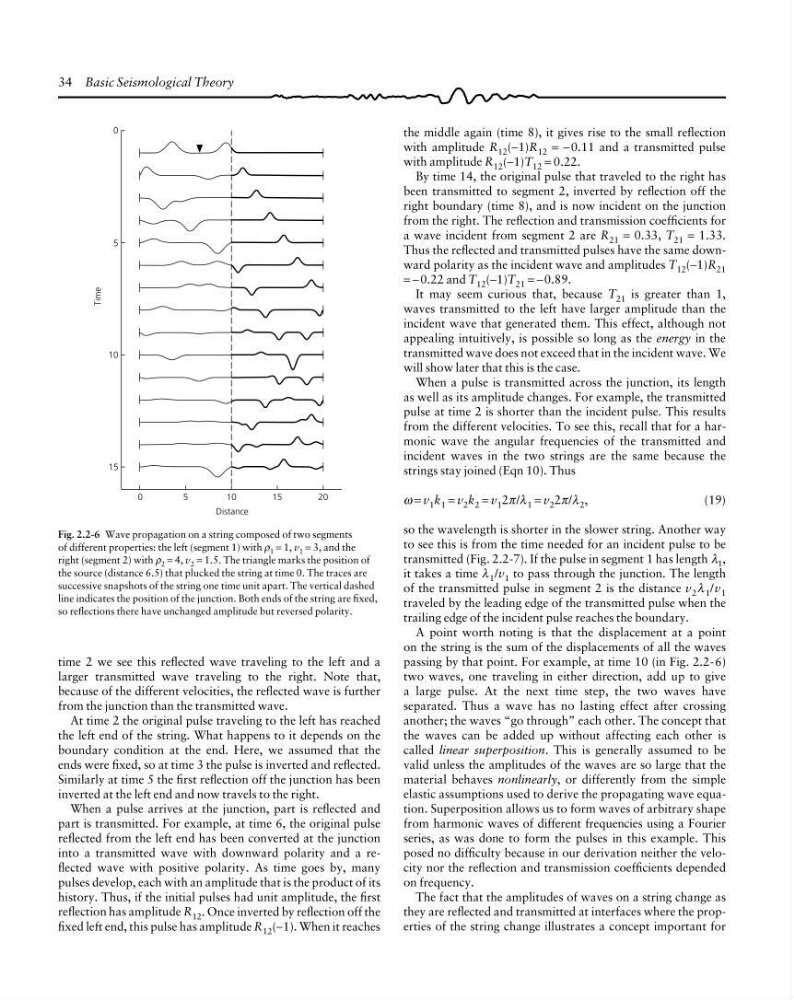
passing by that point. For example, at time 10 (in Fig. 2.2-6)
two waves, one traveling in either direction, add up to give
a large pulse. At the next time step, the two waves have
separated. Thus a wave has no lasting effect after crossing
another; the waves “go through” each other. The concept that
the waves can be added up without affecting each other is
called linear superposition. This is generally assumed to be
valid unless the amplitudes of the waves are so large that the
material behaves nonlinearly, or differently from the simple
elastic assumptions used to derive the propagating wave equation. Superposition allows us to form waves of arbitrary shape
from harmonic waves of different frequencies using a Fourier
series, as was done to form the pulses in this example. This
posed no difficulty because in our derivation neither the velocity nor the reflection and transmission coefficients depended
on frequency.
The fact that the amplitudes of waves on a string change as
they are reflected and transmitted at interfaces where the properties of the string change illustrates a concept important for
Fig. 2.2-6 Wave propagation on a string composed of two segments
of different properties: the left (segment 1) with ρ 1 = 1, v 1 = 3, and the
right (segment 2) with ρ 2 = 4, v 2 = 1.5. The triangle marks the position of
the source (distance 6.5) that plucked the string at time 0. The traces are
successive snapshots of the string one time unit apart. The vertical dashed
line indicates the position of the junction. Both ends of the string are fixed,
so reflections there have unchanged amplitude but reversed polarity.
Time
0
0
Distance
5
1 0
1 5
2 0
5
10
15
time 2 we see this reflected wave traveling to the left and a
larger transmitted wave traveling to the right. Note that,
because of the different velocities, the reflected wave is further
from the junction than the transmitted wave.
At time 2 the original pulse traveling to the left has reached
the left end of the string. What happens to it depends on the
boundary condition at the end. Here, we assumed that the
ends were fixed, so at time 3 the pulse is inverted and reflected.
Similarly at time 5 the first reflection off the junction has been
inverted at the left end and now travels to the right.
When a pulse arrives at the junction, part is reflected and
part is transmitted. For example, at time 6, the original pulse
reflected from the left end has been converted at the junction
into a transmitted wave with downward polarity and a reflected wave with positive polarity. As time goes by, many
pulses develop, each with an amplitude that is the product of its
history. Thus, if the initial pulses had unit amplitude, the first
reflection has amplitude R 12 . Once inverted by reflection off the
fixed left end, this pulse has amplitude R 12 (−1). When it reaches
the middle again (time 8), it gives rise to the small reflection
with amplitude R 12 (−1)R 12 = −0.11 and a transmitted pulse
with amplitude R 12 (−1)T 12 = 0.22.
By time 14, the original pulse that traveled to the right has
been transmitted to segment 2, inverted by reflection off the
right boundary (time 8), and is now incident on the junction
from the right. The reflection and transmission coefficients for
a wave incident from segment 2 are R 21 = 0.33, T 21 = 1.33.
Thus the reflected and transmitted pulses have the same downward polarity as the incident wave and amplitudes T 12 (−1)R 21
= −0.22 and T 12 (−1)T 21 = −0.89.
It may seem curious that, because T 21 is greater than 1,
waves transmitted to the left have larger amplitude than the
incident wave that generated them. This effect, although not
appealing intuitively, is possible so long as the energy in the
transmitted wave does not exceed that in the incident wave. We
will show later that this is the case.
When a pulse is transmitted across the junction, its length
as well as its amplitude changes. For example, the transmitted
pulse at time 2 is shorter than the incident pulse. This results
from the different velocities. To see this, recall that for a harmonic wave the angular frequencies of the transmitted and
incident waves in the two strings are the same because the
strings stay joined (Eqn 10). Thus
ω = v 1 k 1 = v 2 k 2 = v 1 2π/λ 1 = v 2 2π/λ 2 ,
(19)
so the wavelength is shorter in the slower string. Another way
to see this is from the time needed for an incident pulse to be
transmitted (Fig. 2.2-7). If the pulse in segment 1 has length λ 1 ,
it takes a time λ 1 /v 1 to pass through the junction. The length
of the transmitted pulse in segment 2 is the distance v 2 λ 1 /v 1
traveled by the leading edge of the transmitted pulse when the
trailing edge of the incident pulse reaches the boundary.
A point worth noting is that the displacement at a point
on the string is the sum of the displacements of all the waves
passing by that point. For example, at time 10 (in Fig. 2.2-6)
two waves, one traveling in either direction, add up to give
a large pulse. At the next time step, the two waves have
separated. Thus a wave has no lasting effect after crossing
another; the waves “go through” each other. The concept that
the waves can be added up without affecting each other is
called linear superposition. This is generally assumed to be
valid unless the amplitudes of the waves are so large that the
material behaves nonlinearly, or differently from the simple
elastic assumptions used to derive the propagating wave equation. Superposition allows us to form waves of arbitrary shape
from harmonic waves of different frequencies using a Fourier
series, as was done to form the pulses in this example. This
posed no difficulty because in our derivation neither the velocity nor the reflection and transmission coefficients depended
on frequency.
The fact that the amplitudes of waves on a string change as
they are reflected and transmitted at interfaces where the properties of the string change illustrates a concept important for
Fig. 2.2-6 Wave propagation on a string composed of two segments
of different properties: the left (segment 1) with ρ 1 = 1, v 1 = 3, and the
right (segment 2) with ρ 2 = 4, v 2 = 1.5. The triangle marks the position of
the source (distance 6.5) that plucked the string at time 0. The traces are
successive snapshots of the string one time unit apart. The vertical dashed
line indicates the position of the junction. Both ends of the string are fixed,
so reflections there have unchanged amplitude but reversed polarity.
Time
0
0
Distance
5
1 0
1 5
2 0
5
10
15
time 2 we see this reflected wave traveling to the left and a
larger transmitted wave traveling to the right. Note that,
because of the different velocities, the reflected wave is further
from the junction than the transmitted wave.
At time 2 the original pulse traveling to the left has reached
the left end of the string. What happens to it depends on the
boundary condition at the end. Here, we assumed that the
ends were fixed, so at time 3 the pulse is inverted and reflected.
Similarly at time 5 the first reflection off the junction has been
inverted at the left end and now travels to the right.
When a pulse arrives at the junction, part is reflected and
part is transmitted. For example, at time 6, the original pulse
reflected from the left end has been converted at the junction
into a transmitted wave with downward polarity and a reflected wave with positive polarity. As time goes by, many
pulses develop, each with an amplitude that is the product of its
history. Thus, if the initial pulses had unit amplitude, the first
reflection has amplitude R 12 . Once inverted by reflection off the
fixed left end, this pulse has amplitude R 12 (−1). When it reaches