

yields a unique solution vector x. For inhomogeneous systems,
computing A
−1 provides a straightforward manner of solving
for the unknown variables x i . For homogeneous systems of
equations, the equation shows that x = 0 if A −1 exists. Thus,
for a homogeneous system to have a nonzero or nontrivial
solution, A must be singular. This occurs if the determinant of
A is zero, implying that some of the rows (or columns) of A are
not linearly independent. If a nontrivial solution of the homogeneous system exists, any constant times that solution is also
a solution.
If the coefficient matrix is singular, the corresponding
inhomogeneous system of equations does not have unique
solutions, and may have none. The existence of A −1 and the
solvability of the equations thus depend on whether the rows
and columns of A are linearly independent. For example, if the
rows are linearly dependent, there are fewer independent equations than unknowns and difficulties result, as discussed in the
context of inverse problems (Chapter 7).
A.4.5 Solving systems of equations on a computer
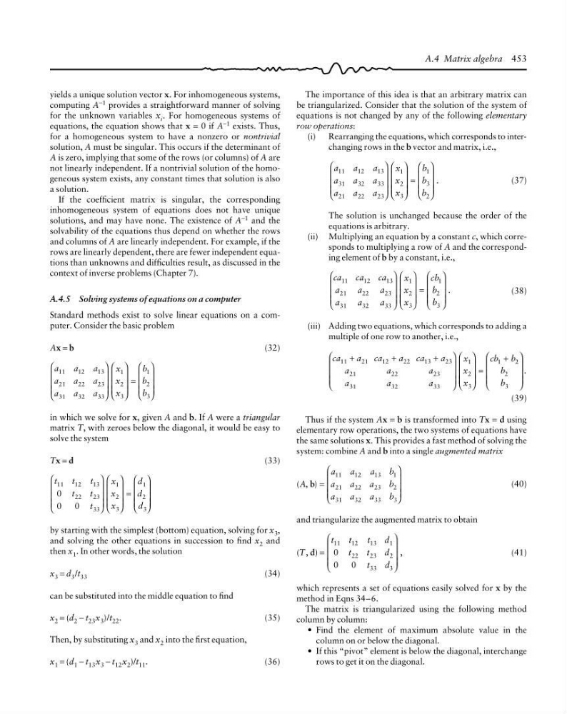
Standard methods exist to solve linear equations on a computer. Consider the basic problem
Ax = b
(32)
a
a
a
a
a
a
a
a
a
x
x
x
b
b
b
11
12
13
21
22
23
31
32
33
1
2
3
1
2
3
⎛
⎝
⎜
⎜
⎜
⎞
⎠
⎟
⎟
⎟
⎛
⎝
⎜
⎜
⎜
⎞
⎠
⎟
⎟
⎟
=
⎛
⎝
⎜
⎜
⎜
⎞
⎠
⎟
⎟
⎟
in which we solve for x, given A and b. If A were a triangular
matrix T, with zeroes below the diagonal, it would be easy to
solve the system
Tx = d
(33)
t
t
t
t
t
t
x
x
x
d
d
d
11
12
13
22
23
33
1
2
3
1
2
3
0
0
0
⎛
⎝
⎜
⎜
⎜
⎞
⎠
⎟
⎟
⎟
⎛
⎝
⎜
⎜
⎜
⎞
⎠
⎟
⎟
⎟
=
⎛
⎝
⎜
⎜
⎜
⎞
⎠
⎟
⎟
⎟
by starting with the simplest (bottom) equation, solving for x 3 ,
and solving the other equations in succession to find x 2 and
then x 1 . In other words, the solution
x 3 = d 3 /t 33
(34)
can be substituted into the middle equation to find
x 2 = (d 2 − t 23 x 3 )/t 22 .
(35)
Then, by substituting x 3 and x 2 into the first equation,
x 1 = (d 1 − t 13 x 3 − t 12 x 2 )/t 11 .
(36)
The importance of this idea is that an arbitrary matrix can
be triangularized. Consider that the solution of the system of
equations is not changed by any of the following elementary
row operations:
(i) Rearranging the equations, which corresponds to interchanging rows in the b vector and matrix, i.e.,
a
a
a
a
a
a
a
a
a
x
x
x
b
b
b
11
12
13
31
32
33
21
22
23
1
2
3
1
3
2
⎛
⎝
⎜
⎜
⎜
⎞
⎠
⎟
⎟
⎟
⎛
⎝
⎜
⎜
⎜
⎞
⎠
⎟
⎟
⎟
=
⎛
⎝
⎜
⎜
⎜
⎞
⎠
⎟
⎟
⎟
.
(37)
The solution is unchanged because the order of the
equations is arbitrary.
(ii) Multiplying an equation by a constant c, which corresponds to multiplying a row of A and the corresponding element of b by a constant, i.e.,
ca
ca
ca
a
a
a
a
a
a
x
x
x
cb
b
b
11
12
13
21
22
23
31
32
33
1
2
3
1
2
3
⎛
⎝
⎜
⎜
⎜
⎞
⎠
⎟
⎟
⎟
⎛
⎝
⎜
⎜
⎜
⎞
⎠
⎟
⎟
⎟
=
⎛
⎝
⎜
⎜
⎜
⎞
⎠
⎟
⎟
⎟
.
(38)
(iii) Adding two equations, which corresponds to adding a
multiple of one row to another, i.e.,
ca
a ca
a ca
a
a
a
a
a
a
a
x
x
x
cb b
b
b
11
21
12
22
13
23
21
22
23
31
32
33
1
2
3
1
2
2
3
+
+
+
⎛
⎝
⎜
⎜
⎜
⎞
⎠
⎟
⎟
⎟
⎛
⎝
⎜
⎜
⎜
⎞
⎠
⎟
⎟
⎟
=
+
⎛
⎝
⎜
⎜
⎜
⎞
⎠
⎟
⎟
⎟
.
(39)
Thus if the system Ax = b is transformed into Tx = d using
elementary row operations, the two systems of equations have
the same solutions x. This provides a fast method of solving the
system: combine A and b into a single augmented matrix
( , )
A
a
a
a
b
a
a
a
b
a
a
a
b
b =
⎛
⎝
⎜
⎜
⎜
⎞
⎠
⎟
⎟
⎟
11
12
13
1
21
22
23
2
31
32
33
3
(40)
and triangularize the augmented matrix to obtain
( , )
,
T
t
t
t
d
t
t
d
t
d
d =
⎛
⎝
⎜
⎜
⎜
⎞
⎠
⎟
⎟
⎟
11
12
13
1
22
23
2
33
3
0
0
0
(41)
which represents a set of equations easily solved for x by the
method in Eqns 34–6.
The matrix is triangularized using the following method
column by column:
• Find the element of maximum absolute value in the
column on or below the diagonal.
• If this “pivot” element is below the diagonal, interchange
rows to get it on the diagonal.
A.4 Matrix algebra 453
computing A
−1 provides a straightforward manner of solving
for the unknown variables x i . For homogeneous systems of
equations, the equation shows that x = 0 if A −1 exists. Thus,
for a homogeneous system to have a nonzero or nontrivial
solution, A must be singular. This occurs if the determinant of
A is zero, implying that some of the rows (or columns) of A are
not linearly independent. If a nontrivial solution of the homogeneous system exists, any constant times that solution is also
a solution.
If the coefficient matrix is singular, the corresponding
inhomogeneous system of equations does not have unique
solutions, and may have none. The existence of A −1 and the
solvability of the equations thus depend on whether the rows
and columns of A are linearly independent. For example, if the
rows are linearly dependent, there are fewer independent equations than unknowns and difficulties result, as discussed in the
context of inverse problems (Chapter 7).
A.4.5 Solving systems of equations on a computer
Standard methods exist to solve linear equations on a computer. Consider the basic problem
Ax = b
(32)
a
a
a
a
a
a
a
a
a
x
x
x
b
b
b
11
12
13
21
22
23
31
32
33
1
2
3
1
2
3
⎛
⎝
⎜
⎜
⎜
⎞
⎠
⎟
⎟
⎟
⎛
⎝
⎜
⎜
⎜
⎞
⎠
⎟
⎟
⎟
=
⎛
⎝
⎜
⎜
⎜
⎞
⎠
⎟
⎟
⎟
in which we solve for x, given A and b. If A were a triangular
matrix T, with zeroes below the diagonal, it would be easy to
solve the system
Tx = d
(33)
t
t
t
t
t
t
x
x
x
d
d
d
11
12
13
22
23
33
1
2
3
1
2
3
0
0
0
⎛
⎝
⎜
⎜
⎜
⎞
⎠
⎟
⎟
⎟
⎛
⎝
⎜
⎜
⎜
⎞
⎠
⎟
⎟
⎟
=
⎛
⎝
⎜
⎜
⎜
⎞
⎠
⎟
⎟
⎟
by starting with the simplest (bottom) equation, solving for x 3 ,
and solving the other equations in succession to find x 2 and
then x 1 . In other words, the solution
x 3 = d 3 /t 33
(34)
can be substituted into the middle equation to find
x 2 = (d 2 − t 23 x 3 )/t 22 .
(35)
Then, by substituting x 3 and x 2 into the first equation,
x 1 = (d 1 − t 13 x 3 − t 12 x 2 )/t 11 .
(36)
The importance of this idea is that an arbitrary matrix can
be triangularized. Consider that the solution of the system of
equations is not changed by any of the following elementary
row operations:
(i) Rearranging the equations, which corresponds to interchanging rows in the b vector and matrix, i.e.,
a
a
a
a
a
a
a
a
a
x
x
x
b
b
b
11
12
13
31
32
33
21
22
23
1
2
3
1
3
2
⎛
⎝
⎜
⎜
⎜
⎞
⎠
⎟
⎟
⎟
⎛
⎝
⎜
⎜
⎜
⎞
⎠
⎟
⎟
⎟
=
⎛
⎝
⎜
⎜
⎜
⎞
⎠
⎟
⎟
⎟
.
(37)
The solution is unchanged because the order of the
equations is arbitrary.
(ii) Multiplying an equation by a constant c, which corresponds to multiplying a row of A and the corresponding element of b by a constant, i.e.,
ca
ca
ca
a
a
a
a
a
a
x
x
x
cb
b
b
11
12
13
21
22
23
31
32
33
1
2
3
1
2
3
⎛
⎝
⎜
⎜
⎜
⎞
⎠
⎟
⎟
⎟
⎛
⎝
⎜
⎜
⎜
⎞
⎠
⎟
⎟
⎟
=
⎛
⎝
⎜
⎜
⎜
⎞
⎠
⎟
⎟
⎟
.
(38)
(iii) Adding two equations, which corresponds to adding a
multiple of one row to another, i.e.,
ca
a ca
a ca
a
a
a
a
a
a
a
x
x
x
cb b
b
b
11
21
12
22
13
23
21
22
23
31
32
33
1
2
3
1
2
2
3
+
+
+
⎛
⎝
⎜
⎜
⎜
⎞
⎠
⎟
⎟
⎟
⎛
⎝
⎜
⎜
⎜
⎞
⎠
⎟
⎟
⎟
=
+
⎛
⎝
⎜
⎜
⎜
⎞
⎠
⎟
⎟
⎟
.
(39)
Thus if the system Ax = b is transformed into Tx = d using
elementary row operations, the two systems of equations have
the same solutions x. This provides a fast method of solving the
system: combine A and b into a single augmented matrix
( , )
A
a
a
a
b
a
a
a
b
a
a
a
b
b =
⎛
⎝
⎜
⎜
⎜
⎞
⎠
⎟
⎟
⎟
11
12
13
1
21
22
23
2
31
32
33
3
(40)
and triangularize the augmented matrix to obtain
( , )
,
T
t
t
t
d
t
t
d
t
d
d =
⎛
⎝
⎜
⎜
⎜
⎞
⎠
⎟
⎟
⎟
11
12
13
1
22
23
2
33
3
0
0
0
(41)
which represents a set of equations easily solved for x by the
method in Eqns 34–6.
The matrix is triangularized using the following method
column by column:
• Find the element of maximum absolute value in the
column on or below the diagonal.
• If this “pivot” element is below the diagonal, interchange
rows to get it on the diagonal.
A.4 Matrix algebra 453