

228 Earthquakes
planes, especially if the plane is far from the vertical, as in the
dip-slip examples shown. In such cases, information about the
waveforms as well as the polarity of the waves is used, as discussed later.
4.2.5 Analytical representation of fault geometry
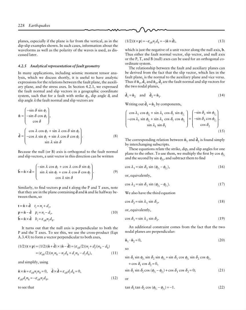
In many applications, including seismic moment tensor analysis, which we discuss shortly, it is useful to have analytic
expressions for the relations between the fault plane, the auxiliary plane, and the stress axes. In Section 4.2.1, we expressed
the fault normal and slip vectors in a geographic coordinate
system, such that for a fault with strike φ f , dip angle δ, and
slip angle λ the fault normal and slip vectors are
4
sin sin
sin cos
cos
,
=
−
−
⎛
⎝
⎜
⎜
⎜
⎞
⎠
⎟
⎟
⎟
δ
φ
δ
φ
δ
f
f
2
cos cos
sin cos sin
cos sin
sin cos cos
sin sin
.
=
+
−
+
⎛
⎝
⎜
⎜ ⎜
⎞
⎠
⎟
⎟ ⎟
λ
φ
λ
δ
φ
λ
φ
λ
δ
φ
λ
δ
f
f
f
f
(8)
Because the null (or B) axis is orthogonal to the fault normal
and slip vectors, a unit vector in this direction can be written
1 = 4 × 2 =
−
+
+
⎛
⎝
⎜
⎜ ⎜
⎞
⎠
⎟
⎟ ⎟
sin cos
cos cos sin
sin sin
cos cos cos
cos sin
.
λ
φ
λ
δ
φ
λ
φ
λ
δ
φ
λ
δ
f
f
f
f
(9)
Similarly, to find vectors p and t along the P and T axes, note
that they are in the plane containing 2 and 4 and lie halfway between them, so
t = 4 + 2 t i = n i + d i ,
p = 4 − 2 p i = n i − d i ,
(10)
1 = 4 × 2 b i = ε ijk n j d k .
It turns out that the null axis is perpendicular to both the
P and the T axes. To see this, we use the cross-product (Eqn
A.3.43) to form a vector perpendicular to both axes,
(1/2)(t × p) = (1/2)(4 + 2) × (4 − 2) = (ε ijk /2)(n j + d j )(n k − d k )
= (ε ijk /2)(n j n k − n j d k + d j n k − d j d k ),
(11)
and simplify, using
4 × 4 = ε ijk n j n k = 0, 2 × 2 = ε ijk d j d k = 0,
ε ijk d j n k = −ε ijk n j d k ,
(12)
to see that
(1/2)(t × p) = −ε ijk n j d k = −(4 × 2),
(13)
which is just the negative of a unit vector along the null axis, b.
Thus either the fault normal vector, slip vector, and null axis
or the P, T, and B (null) axes can be used for an orthogonal coordinate system.
The relationship between the fault and auxiliary planes can
be derived from the fact that the slip vector, which lies in the
fault plane, is the normal to the auxiliary plane and vice versa.
Thus if 4 1 , 2 1 and 4 2 , 2 2 are the fault normal and slip vectors for
the two nodal planes,
2 1 = 4 2 and 2 2 = 4 1 .
(14)
Writing out 2 1 = 4 2 by components,
cos cos
sin
cos sin
cos sin
sin cos cos
sin sin
sin sin
sin cos
cos
.
λ
φ
λ
δ
φ
λ
φ
λ
δ
φ
λ
δ
δ
φ
δ
φ
δ
1
1
1
1
1
1
1
1
2
2
2
1
1
1
1
2
2
f
f
f
f
f
f
+
−
+
⎛
⎝
⎜
⎜
⎜
⎞
⎠
⎟
⎟
⎟
=
−
−
⎛
⎝
⎜
⎜
⎜
⎞
⎠
⎟
⎟
⎟
(15)
The corresponding relation between 4 1 and 2 2 is found simply
by interchanging subscripts.
These equations relate the strike, dip, and slip angles for one
plane to the other. To use them, we multiply the first by cos φ f1
and the second by sin φ f1 , and subtract them to find
cos λ 1 = sin δ 2 sin (φ f1 − φ f2 ),
(16)
or, equivalently,
cos λ 2 = sin δ 1 sin (φ f2 − φ f 1 ).
(17)
We also have the third equation
cos δ 2 = sin λ 1 sin δ 1 ,
(18)
or, equivalently,
cos δ 1 = sin λ 2 sin δ 2 .
(19)
An additional constraint comes from the fact that the two
nodal planes are perpendicular:
4 1 · 4 2 = 0,
(20)
so
sin δ 1 sin φ f1 sin δ 2 sin φ f2 + sin δ 1 cos φ f1 sin δ 2 cos φ f2
+ cos δ 1 cos δ 2 = 0,
sin δ 1 sin δ 2 cos (φ f1 − φ f2 ) + cos δ 1 cos δ 2 = 0;
(21)
or
tan δ 1 tan δ 2 cos (φ f1 − φ f2 ) = −1.
(22)
planes, especially if the plane is far from the vertical, as in the
dip-slip examples shown. In such cases, information about the
waveforms as well as the polarity of the waves is used, as discussed later.
4.2.5 Analytical representation of fault geometry
In many applications, including seismic moment tensor analysis, which we discuss shortly, it is useful to have analytic
expressions for the relations between the fault plane, the auxiliary plane, and the stress axes. In Section 4.2.1, we expressed
the fault normal and slip vectors in a geographic coordinate
system, such that for a fault with strike φ f , dip angle δ, and
slip angle λ the fault normal and slip vectors are
4
sin sin
sin cos
cos
,
=
−
−
⎛
⎝
⎜
⎜
⎜
⎞
⎠
⎟
⎟
⎟
δ
φ
δ
φ
δ
f
f
2
cos cos
sin cos sin
cos sin
sin cos cos
sin sin
.
=
+
−
+
⎛
⎝
⎜
⎜ ⎜
⎞
⎠
⎟
⎟ ⎟
λ
φ
λ
δ
φ
λ
φ
λ
δ
φ
λ
δ
f
f
f
f
(8)
Because the null (or B) axis is orthogonal to the fault normal
and slip vectors, a unit vector in this direction can be written
1 = 4 × 2 =
−
+
+
⎛
⎝
⎜
⎜ ⎜
⎞
⎠
⎟
⎟ ⎟
sin cos
cos cos sin
sin sin
cos cos cos
cos sin
.
λ
φ
λ
δ
φ
λ
φ
λ
δ
φ
λ
δ
f
f
f
f
(9)
Similarly, to find vectors p and t along the P and T axes, note
that they are in the plane containing 2 and 4 and lie halfway between them, so
t = 4 + 2 t i = n i + d i ,
p = 4 − 2 p i = n i − d i ,
(10)
1 = 4 × 2 b i = ε ijk n j d k .
It turns out that the null axis is perpendicular to both the
P and the T axes. To see this, we use the cross-product (Eqn
A.3.43) to form a vector perpendicular to both axes,
(1/2)(t × p) = (1/2)(4 + 2) × (4 − 2) = (ε ijk /2)(n j + d j )(n k − d k )
= (ε ijk /2)(n j n k − n j d k + d j n k − d j d k ),
(11)
and simplify, using
4 × 4 = ε ijk n j n k = 0, 2 × 2 = ε ijk d j d k = 0,
ε ijk d j n k = −ε ijk n j d k ,
(12)
to see that
(1/2)(t × p) = −ε ijk n j d k = −(4 × 2),
(13)
which is just the negative of a unit vector along the null axis, b.
Thus either the fault normal vector, slip vector, and null axis
or the P, T, and B (null) axes can be used for an orthogonal coordinate system.
The relationship between the fault and auxiliary planes can
be derived from the fact that the slip vector, which lies in the
fault plane, is the normal to the auxiliary plane and vice versa.
Thus if 4 1 , 2 1 and 4 2 , 2 2 are the fault normal and slip vectors for
the two nodal planes,
2 1 = 4 2 and 2 2 = 4 1 .
(14)
Writing out 2 1 = 4 2 by components,
cos cos
sin
cos sin
cos sin
sin cos cos
sin sin
sin sin
sin cos
cos
.
λ
φ
λ
δ
φ
λ
φ
λ
δ
φ
λ
δ
δ
φ
δ
φ
δ
1
1
1
1
1
1
1
1
2
2
2
1
1
1
1
2
2
f
f
f
f
f
f
+
−
+
⎛
⎝
⎜
⎜
⎜
⎞
⎠
⎟
⎟
⎟
=
−
−
⎛
⎝
⎜
⎜
⎜
⎞
⎠
⎟
⎟
⎟
(15)
The corresponding relation between 4 1 and 2 2 is found simply
by interchanging subscripts.
These equations relate the strike, dip, and slip angles for one
plane to the other. To use them, we multiply the first by cos φ f1
and the second by sin φ f1 , and subtract them to find
cos λ 1 = sin δ 2 sin (φ f1 − φ f2 ),
(16)
or, equivalently,
cos λ 2 = sin δ 1 sin (φ f2 − φ f 1 ).
(17)
We also have the third equation
cos δ 2 = sin λ 1 sin δ 1 ,
(18)
or, equivalently,
cos δ 1 = sin λ 2 sin δ 2 .
(19)
An additional constraint comes from the fact that the two
nodal planes are perpendicular:
4 1 · 4 2 = 0,
(20)
so
sin δ 1 sin φ f1 sin δ 2 sin φ f2 + sin δ 1 cos φ f1 sin δ 2 cos φ f2
+ cos δ 1 cos δ 2 = 0,
sin δ 1 sin δ 2 cos (φ f1 − φ f2 ) + cos δ 1 cos δ 2 = 0;
(21)
or
tan δ 1 tan δ 2 cos (φ f1 − φ f2 ) = −1.
(22)