

τ
m
=
2
s
Q
ScS
10 000
10
Normal
modes
Long-period
body waves
Short-period
body waves
Frequency (Hz)
1
.1
.01
.001
1000
100
10
0 . 5
1
0 . 2
0 . 1
3.7 Attenuation and anelasticity 193
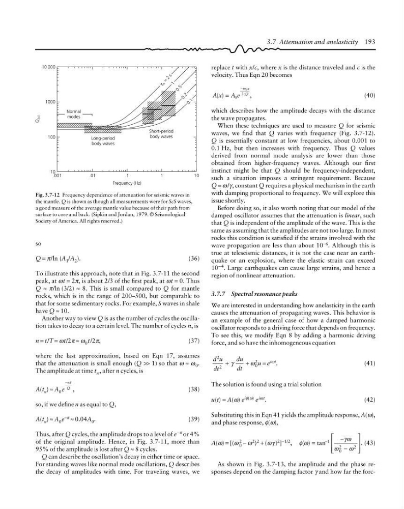
Fig. 3.7-12 Frequency dependence of attenuation for seismic waves in
the mantle. Q is shown as though all measurements were for ScS waves,
a good measure of the average mantle value because of their path from
surface to core and back. (Sipkin and Jordan, 1979. © Seismological
Society of America. All rights reserved.)
so
Q = π/ln (A 1 /A 2 ).
(36)
To illustrate this approach, note that in Fig. 3.7-11 the second
peak, at ωt = 2π, is about 2/3 of the first peak, at ωt = 0. Thus
Q ≈ π/ln (3/2) ≈ 8. This is small compared to Q for mantle
rocks, which is in the range of 200–500, but comparable to
that for some sedimentary rocks. For example, S waves in shale
have Q ≈ 10.
Another way to view Q is as the number of cycles the oscillation takes to decay to a certain level. The number of cycles n, is
n = t/T = ωt/2π ≈ ω 0 t/2π,
(37)
where the last approximation, based on Eqn 17, assumes
that the attenuation is small enough (Q >> 1) so that ω ≈ ω 0 .
The amplitude at time t n , after n cycles, is
A(t n ) ≈ A 0 e
n
Q
− π
,
(38)
so, if we define n as equal to Q,
A(t n ) ≈ A 0 e −π ≈ 0.04A 0 .
(39)
Thus, after Q cycles, the amplitude drops to a level of e
−π or 4%
of the original amplitude. Hence, in Fig. 3.7-11, more than
95% of the amplitude is lost after Q ≈ 8 cycles.
Q can describe the oscillation’s decay in either time or space.
For standing waves like normal mode oscillations, Q describes
the decay of amplitudes with time. For traveling waves, we
replace t with x/c, where x is the distance traveled and c is the
velocity. Thus Eqn 20 becomes
A x A e
x
cQ
( )
,
=
−
0
2
0
ω
(40)
which describes how the amplitude decays with the distance
the wave propagates.
When these techniques are used to measure Q for seismic
waves, we find that Q varies with frequency (Fig. 3.7-12).
Q is essentially constant at low frequencies, about 0.001 to
0.1 Hz, but then increases with frequency. Thus Q values
derived from normal mode analysis are lower than those
obtained from higher-frequency waves. Although our first
instinct might be that Q should be frequency-independent,
such a situation imposes a stringent requirement. Because
Q = ω /γ, constant Q requires a physical mechanism in the earth
with damping proportional to frequency. We will explore this
issue shortly.
Before doing so, it also worth noting that our model of the
damped oscillator assumes that the attenuation is linear, such
that Q is independent of the amplitude of the wave. This is the
same as assuming that the amplitudes are not too large. In most
rocks this condition is satisfied if the strains involved with the
wave propagation are less than about 10 −6 . Although this is
true at teleseismic distances, it is not the case near an earthquake or an explosion, where the elastic strain can exceed
10 − 4 . Large earthquakes can cause large strains, and hence a
region of nonlinear attenuation.
3.7.7 Spectral resonance peaks
We are interested in understanding how anelasticity in the earth
causes the attenuation of propagating waves. This behavior is
an example of the general case of how a damped harmonic
oscillator responds to a driving force that depends on frequency.
To see this, we modify Eqn 8 by adding a harmonic driving
force, and so have the inhomogeneous equation
d u
dt
du
dt
2
2
+ γ
+ ω 2
0 u = e iωt .
(41)
The solution is found using a trial solution
u(t) = A(ω) e iφ(ω) e iωt .
(42)
Substituting this in Eqn 41 yields the amplitude response, A(ω),
and phase response, φ(ω),
A(ω) = [(ω 2
0 − ω 2 ) 2 + (ωγ ) 2 ] −1/2 , φ ω
γω
ω
ω
( ) tan
.
=
−
−
⎡
⎣
⎢
⎢
⎤
⎦
⎥
⎥
−1
0
2
2
(43)
As shown in Fig. 3.7-13, the amplitude and the phase responses depend on the damping factor γ and how far the forc-
m
=
2
s
Q
ScS
10 000
10
Normal
modes
Long-period
body waves
Short-period
body waves
Frequency (Hz)
1
.1
.01
.001
1000
100
10
0 . 5
1
0 . 2
0 . 1
3.7 Attenuation and anelasticity 193
Fig. 3.7-12 Frequency dependence of attenuation for seismic waves in
the mantle. Q is shown as though all measurements were for ScS waves,
a good measure of the average mantle value because of their path from
surface to core and back. (Sipkin and Jordan, 1979. © Seismological
Society of America. All rights reserved.)
so
Q = π/ln (A 1 /A 2 ).
(36)
To illustrate this approach, note that in Fig. 3.7-11 the second
peak, at ωt = 2π, is about 2/3 of the first peak, at ωt = 0. Thus
Q ≈ π/ln (3/2) ≈ 8. This is small compared to Q for mantle
rocks, which is in the range of 200–500, but comparable to
that for some sedimentary rocks. For example, S waves in shale
have Q ≈ 10.
Another way to view Q is as the number of cycles the oscillation takes to decay to a certain level. The number of cycles n, is
n = t/T = ωt/2π ≈ ω 0 t/2π,
(37)
where the last approximation, based on Eqn 17, assumes
that the attenuation is small enough (Q >> 1) so that ω ≈ ω 0 .
The amplitude at time t n , after n cycles, is
A(t n ) ≈ A 0 e
n
Q
− π
,
(38)
so, if we define n as equal to Q,
A(t n ) ≈ A 0 e −π ≈ 0.04A 0 .
(39)
Thus, after Q cycles, the amplitude drops to a level of e
−π or 4%
of the original amplitude. Hence, in Fig. 3.7-11, more than
95% of the amplitude is lost after Q ≈ 8 cycles.
Q can describe the oscillation’s decay in either time or space.
For standing waves like normal mode oscillations, Q describes
the decay of amplitudes with time. For traveling waves, we
replace t with x/c, where x is the distance traveled and c is the
velocity. Thus Eqn 20 becomes
A x A e
x
cQ
( )
,
=
−
0
2
0
ω
(40)
which describes how the amplitude decays with the distance
the wave propagates.
When these techniques are used to measure Q for seismic
waves, we find that Q varies with frequency (Fig. 3.7-12).
Q is essentially constant at low frequencies, about 0.001 to
0.1 Hz, but then increases with frequency. Thus Q values
derived from normal mode analysis are lower than those
obtained from higher-frequency waves. Although our first
instinct might be that Q should be frequency-independent,
such a situation imposes a stringent requirement. Because
Q = ω /γ, constant Q requires a physical mechanism in the earth
with damping proportional to frequency. We will explore this
issue shortly.
Before doing so, it also worth noting that our model of the
damped oscillator assumes that the attenuation is linear, such
that Q is independent of the amplitude of the wave. This is the
same as assuming that the amplitudes are not too large. In most
rocks this condition is satisfied if the strains involved with the
wave propagation are less than about 10 −6 . Although this is
true at teleseismic distances, it is not the case near an earthquake or an explosion, where the elastic strain can exceed
10 − 4 . Large earthquakes can cause large strains, and hence a
region of nonlinear attenuation.
3.7.7 Spectral resonance peaks
We are interested in understanding how anelasticity in the earth
causes the attenuation of propagating waves. This behavior is
an example of the general case of how a damped harmonic
oscillator responds to a driving force that depends on frequency.
To see this, we modify Eqn 8 by adding a harmonic driving
force, and so have the inhomogeneous equation
d u
dt
du
dt
2
2
+ γ
+ ω 2
0 u = e iωt .
(41)
The solution is found using a trial solution
u(t) = A(ω) e iφ(ω) e iωt .
(42)
Substituting this in Eqn 41 yields the amplitude response, A(ω),
and phase response, φ(ω),
A(ω) = [(ω 2
0 − ω 2 ) 2 + (ωγ ) 2 ] −1/2 , φ ω
γω
ω
ω
( ) tan
.
=
−
−
⎡
⎣
⎢
⎢
⎤
⎦
⎥
⎥
−1
0
2
2
(43)
As shown in Fig. 3.7-13, the amplitude and the phase responses depend on the damping factor γ and how far the forc-