

6
1 Molecules and Intermolecular Interactions
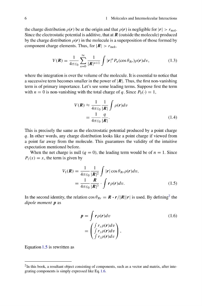
the charge distribution ρ(r) be at the origin and that ρ(r) is negligible for |r| > r mol .
Since the electrostatic potential is additive, that at R (outside the molecule) produced
by the charge distribution ρ(r) in the molecule is a superposition of those formed by
component charge elements. Thus, for |R| > r mol ,
V (R) =
1
4πε 0
∞
n=0
1
|R| n+1
|r|
n P n (cos θ Rr )ρ(r)dv,
(1.3)
where the integration is over the volume of the molecule. It is essential to notice that
a successive term becomes smaller in the power of |R|. Thus, the first non-vanishing
term is of primary importance. Let’s see some leading terms. Suppose first the term
with n = 0 is non-vanishing with the total charge of q. Since P 0 (·) = 1,
V (R) ≈
1
4πε 0
1
|R|
ρ(r)dv
=
1
4πε 0
q
|R|
.
(1.4)
This is precisely the same as the electrostatic potential produced by a point charge
q. In other words, any charge distribution looks like a point charge if viewed from
a point far away from the molecule. This guarantees the validity of the intuitive
expectation mentioned before.
When the net charge is null (q = 0), the leading term would be of n = 1. Since
P 1 (x) = x, the term is given by
V 1 (R) =
1
4πε 0
1
|R| 2
|r| cos θ Rr ρ(r)dv,
=
1
4πε 0
R
|R| 3 ·
rρ(r)dv.
(1.5)
In the second identity, the relation cos θ Rr = R · r/|R||r| is used. By defining
2 the
dipole moment p as
p =
rρ(r)dv
(1.6)
=
⎛
⎝
r x ρ(r)dv
r y ρ(r)dv
r z ρ(r)dv
⎞
⎠ ,
Equation 1.5 is rewritten as
2 In this book, a resultant object consisting of components, such as a vector and matrix, after integrating components is simply expressed like Eq. 1.6.
1 Molecules and Intermolecular Interactions
the charge distribution ρ(r) be at the origin and that ρ(r) is negligible for |r| > r mol .
Since the electrostatic potential is additive, that at R (outside the molecule) produced
by the charge distribution ρ(r) in the molecule is a superposition of those formed by
component charge elements. Thus, for |R| > r mol ,
V (R) =
1
4πε 0
∞
n=0
1
|R| n+1
|r|
n P n (cos θ Rr )ρ(r)dv,
(1.3)
where the integration is over the volume of the molecule. It is essential to notice that
a successive term becomes smaller in the power of |R|. Thus, the first non-vanishing
term is of primary importance. Let’s see some leading terms. Suppose first the term
with n = 0 is non-vanishing with the total charge of q. Since P 0 (·) = 1,
V (R) ≈
1
4πε 0
1
|R|
ρ(r)dv
=
1
4πε 0
q
|R|
.
(1.4)
This is precisely the same as the electrostatic potential produced by a point charge
q. In other words, any charge distribution looks like a point charge if viewed from
a point far away from the molecule. This guarantees the validity of the intuitive
expectation mentioned before.
When the net charge is null (q = 0), the leading term would be of n = 1. Since
P 1 (x) = x, the term is given by
V 1 (R) =
1
4πε 0
1
|R| 2
|r| cos θ Rr ρ(r)dv,
=
1
4πε 0
R
|R| 3 ·
rρ(r)dv.
(1.5)
In the second identity, the relation cos θ Rr = R · r/|R||r| is used. By defining
2 the
dipole moment p as
p =
rρ(r)dv
(1.6)
=
⎛
⎝
r x ρ(r)dv
r y ρ(r)dv
r z ρ(r)dv
⎞
⎠ ,
Equation 1.5 is rewritten as
2 In this book, a resultant object consisting of components, such as a vector and matrix, after integrating components is simply expressed like Eq. 1.6.