

92
5 Lattice Dynamics of Molecular Crystals
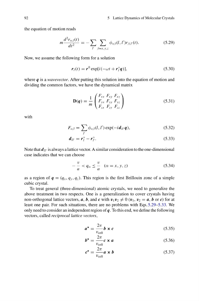
the equation of motion reads
m
d
2 r α.l (t)
dt 2 = −
l
β=x,y,z
φ αβ (l, l
)r β,l (t).
(5.29)
Now, we assume the following form for a solution
r l (t) = r
0 exp[i(−ωt + r
◦
l q)],
(5.30)
where q is a wavevector. After putting this solution into the equation of motion and
dividing the common factors, we have the dynamical matrix
D(q) =
1
m
⎛
⎝
F xx F xy F xz
F yx F yy F yz
F zx F zy F zz
⎞
⎠
(5.31)
with
F αβ =
l
φ αβ (l, l
) exp(−i d ll q),
(5.32)
d ll = r
◦
l − r
◦
l .
(5.33)
Note that d ll is always a lattice vector. A similar consideration to the one-dimensional
case indicates that we can choose
−
π
a
< q α ≤
π
a
(α = x, y, z)
(5.34)
as a region of q = (q x , q y , q z ). This region is the first Brillouin zone of a simple
cubic crystal.
To treat general (three-dimensional) atomic crystals, we need to generalize the
above treatment in two respects. One is a generalization to cover crystals having
non-orthogonal lattice vectors, a, b, and c with v 1 v 2 = 0 (v 1 , v 2 = a, b or c) for at
least one pair. For such situations, there are no problems with Eqs. 5.29–5.33. We
only need to consider an independent region of q. To this end, we define the following
vectors, called reciprocal lattice vectors,
a
∗
=
2π
v cell
b × c
(5.35)
b
∗
=
2π
v cell
c × a
(5.36)
c
∗
=
2π
v cell
a × b
(5.37)
5 Lattice Dynamics of Molecular Crystals
the equation of motion reads
m
d
2 r α.l (t)
dt 2 = −
l
β=x,y,z
φ αβ (l, l
)r β,l (t).
(5.29)
Now, we assume the following form for a solution
r l (t) = r
0 exp[i(−ωt + r
◦
l q)],
(5.30)
where q is a wavevector. After putting this solution into the equation of motion and
dividing the common factors, we have the dynamical matrix
D(q) =
1
m
⎛
⎝
F xx F xy F xz
F yx F yy F yz
F zx F zy F zz
⎞
⎠
(5.31)
with
F αβ =
l
φ αβ (l, l
) exp(−i d ll q),
(5.32)
d ll = r
◦
l − r
◦
l .
(5.33)
Note that d ll is always a lattice vector. A similar consideration to the one-dimensional
case indicates that we can choose
−
π
a
< q α ≤
π
a
(α = x, y, z)
(5.34)
as a region of q = (q x , q y , q z ). This region is the first Brillouin zone of a simple
cubic crystal.
To treat general (three-dimensional) atomic crystals, we need to generalize the
above treatment in two respects. One is a generalization to cover crystals having
non-orthogonal lattice vectors, a, b, and c with v 1 v 2 = 0 (v 1 , v 2 = a, b or c) for at
least one pair. For such situations, there are no problems with Eqs. 5.29–5.33. We
only need to consider an independent region of q. To this end, we define the following
vectors, called reciprocal lattice vectors,
a
∗
=
2π
v cell
b × c
(5.35)
b
∗
=
2π
v cell
c × a
(5.36)
c
∗
=
2π
v cell
a × b
(5.37)