

R
@C
@t ¼
@
@x i
D ij
@C
@x j
À
@
@x i
u i C
ð Þ x; y; z 2 X; t ! 0
Cðx; y; z; tÞ t¼0
j ¼ C 0 ðx; y; zÞ
x; y; z 2 X
Cðx; y; z; tÞ C 1
j ¼ C 1 ðx; y; z; tÞ x; y; z 2 C 1 ; t ! 0
8
> <
> :
where X—vadose region; C—concentration of pollutant components (mg/L),
C = C (x, y, z, t); u i —actual flow velocities in three directions can be obtained
through the groundwater flow model (m/d); D ij —9 components of hydrodynamic
dispersion tensor (m
2 /d); h—effective porosity; q b —dry bulk density of rock and
soil of aquifer; C 0 (x, y, z)—initial concentration of pollutant components (mg/L);
C 1 —Dirichlet boundary condition; C 1 (x, y, z, t)—boundary value of concentration
under the Dirichlet boundary condition, namely concentration value at the boundary
is known (mg/L).
③ Numerical model for migration of pollutes in groundwater
I. Mesh generation in simulation area
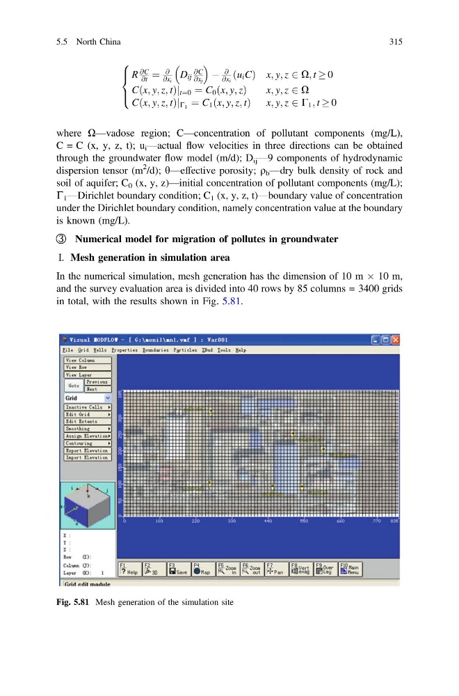
In the numerical simulation, mesh generation has the dimension of 10 m  10 m,
and the survey evaluation area is divided into 40 rows by 85 columns = 3400 grids
in total, with the results shown in Fig. 5.81.
Fig. 5.81 Mesh generation of the simulation site
5.5 North China
315
@C
@t ¼
@
@x i
D ij
@C
@x j
À
@
@x i
u i C
ð Þ x; y; z 2 X; t ! 0
Cðx; y; z; tÞ t¼0
j ¼ C 0 ðx; y; zÞ
x; y; z 2 X
Cðx; y; z; tÞ C 1
j ¼ C 1 ðx; y; z; tÞ x; y; z 2 C 1 ; t ! 0
8
> <
> :
where X—vadose region; C—concentration of pollutant components (mg/L),
C = C (x, y, z, t); u i —actual flow velocities in three directions can be obtained
through the groundwater flow model (m/d); D ij —9 components of hydrodynamic
dispersion tensor (m
2 /d); h—effective porosity; q b —dry bulk density of rock and
soil of aquifer; C 0 (x, y, z)—initial concentration of pollutant components (mg/L);
C 1 —Dirichlet boundary condition; C 1 (x, y, z, t)—boundary value of concentration
under the Dirichlet boundary condition, namely concentration value at the boundary
is known (mg/L).
③ Numerical model for migration of pollutes in groundwater
I. Mesh generation in simulation area
In the numerical simulation, mesh generation has the dimension of 10 m  10 m,
and the survey evaluation area is divided into 40 rows by 85 columns = 3400 grids
in total, with the results shown in Fig. 5.81.
Fig. 5.81 Mesh generation of the simulation site
5.5 North China
315