

16 Production Planning of Remanufactured Products with Inventory …
225
the growth stage (a), the number of newly manufactured products required during
the stage is remarkable to meet the increasing demand. Therefore, a large number of
products are manufactured at a single ordering of new manufacture when K M has a
small value, which leads to an increase in the total cost due to excessive inventory.
Also, when the number of ordering has a small value the total cost has a small
variation to all K M ; however, the variation of the total cost becomes significant as
the number of ordering becomes large. In the maturity stage (b), the increase of
demand terminates, and the collection of used products increases. Therefore, the
number of newly manufactured products required decreases. Accordingly, the total
cost has relatively small values, even if the number of ordering is reduced. During
the decline stage (c), the collecting quantity increases, and the demand quantity
decreases. Therefore, the newly manufactured product quantity required is further
reduced. Moreover, even if all the necessary products are newly manufactured in
single ordering (the number of ordering is one), excessive inventory does not occur.
Figures 16.3 and 16.4 show that as K M and h F change, different characteristics
appear in each stage. The effect of K M in Fig. 16.3 increases when the number of
ordering has a large value; however, the effect of h F increases when the number
of ordering is small. Consequently, it is crucial to focus on the individual values
of K M and h F as well as the ratio of the two values for the production planning of
remanufactured products.
16.4 Influence of Prediction Accuracy of Demand
and Collection on the Total Cost
In this section, the influence on the total cost is examined under the condition that
the actual values of the demand quantity and the collecting quantity differ from
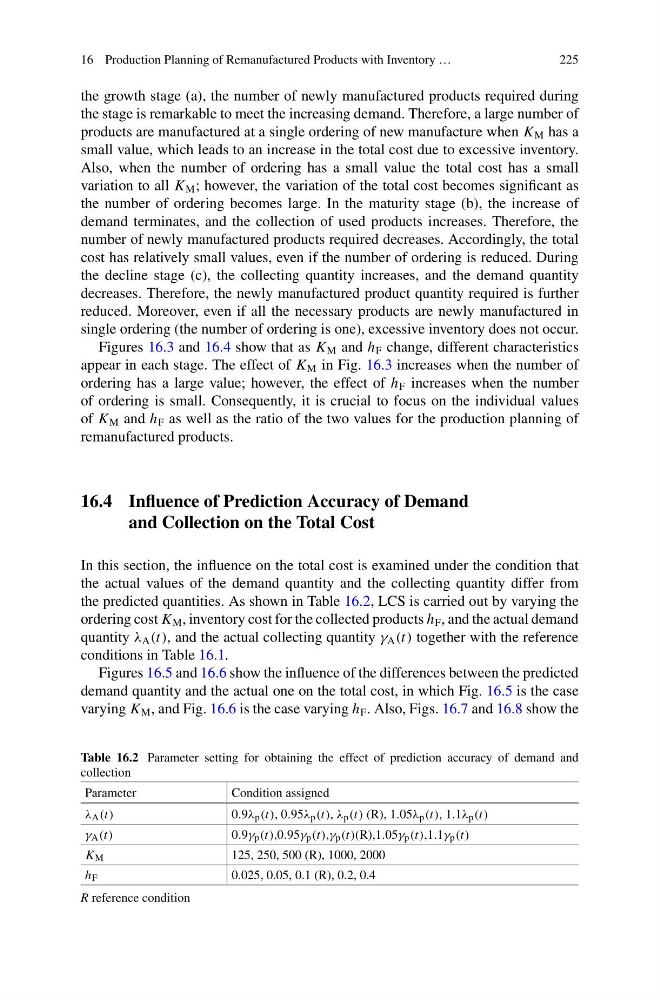
the predicted quantities. As shown in Table 16.2, LCS is carried out by varying the
ordering cost K M , inventory cost for the collected products h F , and the actual demand
quantity λ A (t), and the actual collecting quantity γ A (t) together with the reference
conditions in Table 16.1.
Figures 16.5 and 16.6 show the influence of the differences between the predicted
demand quantity and the actual one on the total cost, in which Fig. 16.5 is the case
varying K M , and Fig. 16.6 is the case varying h F . Also, Figs. 16.7 and 16.8 show the
Table 16.2 Parameter setting for obtaining the effect of prediction accuracy of demand and
collection
Parameter
Condition assigned
λ A (t)
0.9λ p (t), 0.95λ p (t), λ p (t) (R), 1.05λ p (t), 1.1λ p (t)
γ A (t)
0.9γ p (t),0.95γ p (t),γ p (t)(R),1.05γ p (t),1.1γ p (t)
K M
125, 250, 500 (R), 1000, 2000
h F
0.025, 0.05, 0.1 (R), 0.2, 0.4
R reference condition
225
the growth stage (a), the number of newly manufactured products required during
the stage is remarkable to meet the increasing demand. Therefore, a large number of
products are manufactured at a single ordering of new manufacture when K M has a
small value, which leads to an increase in the total cost due to excessive inventory.
Also, when the number of ordering has a small value the total cost has a small
variation to all K M ; however, the variation of the total cost becomes significant as
the number of ordering becomes large. In the maturity stage (b), the increase of
demand terminates, and the collection of used products increases. Therefore, the
number of newly manufactured products required decreases. Accordingly, the total
cost has relatively small values, even if the number of ordering is reduced. During
the decline stage (c), the collecting quantity increases, and the demand quantity
decreases. Therefore, the newly manufactured product quantity required is further
reduced. Moreover, even if all the necessary products are newly manufactured in
single ordering (the number of ordering is one), excessive inventory does not occur.
Figures 16.3 and 16.4 show that as K M and h F change, different characteristics
appear in each stage. The effect of K M in Fig. 16.3 increases when the number of
ordering has a large value; however, the effect of h F increases when the number
of ordering is small. Consequently, it is crucial to focus on the individual values
of K M and h F as well as the ratio of the two values for the production planning of
remanufactured products.
16.4 Influence of Prediction Accuracy of Demand
and Collection on the Total Cost
In this section, the influence on the total cost is examined under the condition that
the actual values of the demand quantity and the collecting quantity differ from
the predicted quantities. As shown in Table 16.2, LCS is carried out by varying the
ordering cost K M , inventory cost for the collected products h F , and the actual demand
quantity λ A (t), and the actual collecting quantity γ A (t) together with the reference
conditions in Table 16.1.
Figures 16.5 and 16.6 show the influence of the differences between the predicted
demand quantity and the actual one on the total cost, in which Fig. 16.5 is the case
varying K M , and Fig. 16.6 is the case varying h F . Also, Figs. 16.7 and 16.8 show the
Table 16.2 Parameter setting for obtaining the effect of prediction accuracy of demand and
collection
Parameter
Condition assigned
λ A (t)
0.9λ p (t), 0.95λ p (t), λ p (t) (R), 1.05λ p (t), 1.1λ p (t)
γ A (t)
0.9γ p (t),0.95γ p (t),γ p (t)(R),1.05γ p (t),1.1γ p (t)
K M
125, 250, 500 (R), 1000, 2000
h F
0.025, 0.05, 0.1 (R), 0.2, 0.4
R reference condition