

transfer area of 1735 m
2 would behave similarly as a horizontal SWM tube (10 m  0.2 m) with 10 SWM cylindrical
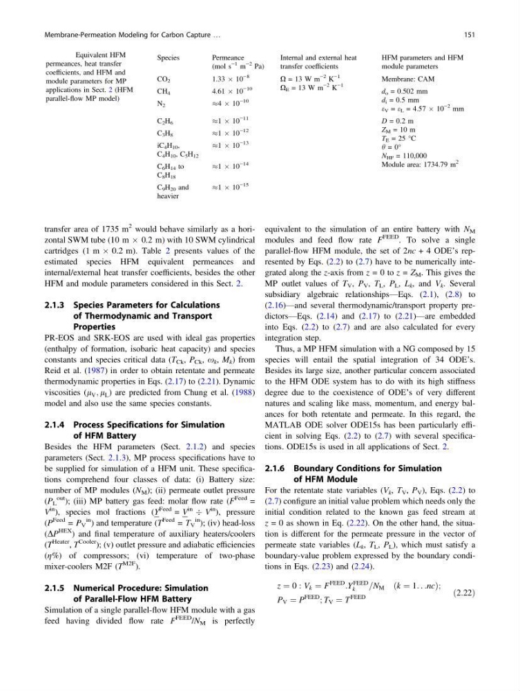
cartridges (1 m  0.2 m). Table 2 presents values of the
estimated species HFM equivalent permeances and
internal/external heat transfer coefficients, besides the other
HFM and module parameters considered in this Sect. 2.
2.1.3 Species Parameters for Calculations
of Thermodynamic and Transport
Properties
PR-EOS and SRK-EOS are used with ideal gas properties
(enthalpy of formation, isobaric heat capacity) and species
constants and species critical data (T Ck , P Ck , x k , M k ) from
Reid et al. (1987) in order to obtain retentate and permeate
thermodynamic properties in Eqs. (2.17) to (2.21). Dynamic
viscosities (l V ; l L ) are predicted from Chung et al. (1988)
model and also use the same species constants.
2.1.4 Process Specifications for Simulation
of HFM Battery
Besides the HFM parameters (Sect. 2.1.2) and species
parameters (Sect. 2.1.3), MP process specifications have to
be supplied for simulation of a HFM unit. These specifications comprehend four classes of data: (i) Battery size:
number of MP modules (N M ); (ii) permeate outlet pressure
(P L
out ); (iii) MP battery gas feed: molar flow rate (F
Feed =
V
in ), species mol fractions (Y
Feed = V
in
Ä V
in
), pressure
(P
Feed = P V
in ) and temperature (T
Feed = T V
in
); (iv) head-loss
(DP
HEX ) and final temperature of auxiliary heaters/coolers
(T
Heater , T
Cooler ); (v) outlet pressure and adiabatic efficiencies
(η%) of compressors; (vi) temperature of two-phase
mixer-coolers M2F (T
M2F ).
2.1.5 Numerical Procedure: Simulation
of Parallel-Flow HFM Battery
Simulation of a single parallel-flow HFM module with a gas
feed having divided flow rate F
FEED /N M is perfectly
equivalent to the simulation of an entire battery with N M
modules and feed flow rate F
FEED . To solve a single
parallel-flow HFM module, the set of 2nc + 4 ODE’s represented by Eqs. (2.2) to (2.7) have to be numerically integrated along the z-axis from z = 0 to z = Z M . This gives the
MP outlet values of T V , P V , T L , P L , L k , and V k . Several
subsidiary algebraic relationships—Eqs. (2.1), (2.8) to
(2.16)—and several thermodynamic/transport property predictors—Eqs. (2.14) and (2.17) to (2.21)—are embedded
into Eqs. (2.2) to (2.7) and are also calculated for every
integration step.
Thus, a MP HFM simulation with a NG composed by 15
species will entail the spatial integration of 34 ODE’s.
Besides its large size, another particular concern associated
to the HFM ODE system has to do with its high stiffness
degree due to the coexistence of ODE’s of very different
natures and scaling like mass, momentum, and energy balances for both retentate and permeate. In this regard, the
MATLAB ODE solver ODE15s has been particularly efficient in solving Eqs. (2.2) to (2.7) with several specifications. ODE15s is used in all applications of Sect. 2.
2.1.6 Boundary Conditions for Simulation
of HFM Module
For the retentate state variables (V k , T V , P V ), Eqs. (2.2) to
(2.7) configure an initial value problem which needs only the
initial condition related to the known gas feed stream at
z = 0 as shown in Eq. (2.22). On the other hand, the situation is different for the permeate pressure in the vector of
permeate state variables (L k , T L , P L ), which must satisfy a
boundary-value problem expressed by the boundary conditions in Eqs. (2.23) and (2.24).
z ¼ 0 : V k ¼ F
FEED
:Y
FEED
k
=N M ðk ¼ 1. . .ncÞ;
P V ¼ P
FEED
; T V ¼ T
FEED
ð2:22Þ
Table 2 Equivalent HFM
permeances, heat transfer
coefficients, and HFM and
module parameters for MP
applications in Sect. 2 (HFM
parallel-flow MP model)
Species
Permeance
(mol s
−1 m
−2 Pa)
Internal and external heat
transfer coefficients
HFM parameters and HFM
module parameters
CO 2
1.33 Â 10
−8
X = 13 W m
−2 K
−1
X E = 13 W m
−2 K
−1
Membrane: CAM
CH 4
4.61 Â 10
−10
d o = 0.502 mm
d i = 0.5 mm
e V = e L = 4.57 Â 10
−2 mm
N 2
%4 Â 10
−10
C 2 H 6
%1 Â 10
−11
D = 0.2 m
Z M = 10 m
T E = 25 °C
h = 0°
N HF = 110,000
Module area: 1734.79 m
2
C 3 H 8
%1 Â 10
−12
iC 4 H 10 ,
C 4 H 10 , C 5 H 12
%1 Â 10
−13
C 6 H 14 to
C 8 H 18
%1 Â 10
−14
C 9 H 20 and
heavier
%1 Â 10
−15
Membrane-Permeation Modeling for Carbon Capture …
151
2 would behave similarly as a horizontal SWM tube (10 m  0.2 m) with 10 SWM cylindrical
cartridges (1 m  0.2 m). Table 2 presents values of the
estimated species HFM equivalent permeances and
internal/external heat transfer coefficients, besides the other
HFM and module parameters considered in this Sect. 2.
2.1.3 Species Parameters for Calculations
of Thermodynamic and Transport
Properties
PR-EOS and SRK-EOS are used with ideal gas properties
(enthalpy of formation, isobaric heat capacity) and species
constants and species critical data (T Ck , P Ck , x k , M k ) from
Reid et al. (1987) in order to obtain retentate and permeate
thermodynamic properties in Eqs. (2.17) to (2.21). Dynamic
viscosities (l V ; l L ) are predicted from Chung et al. (1988)
model and also use the same species constants.
2.1.4 Process Specifications for Simulation
of HFM Battery
Besides the HFM parameters (Sect. 2.1.2) and species
parameters (Sect. 2.1.3), MP process specifications have to
be supplied for simulation of a HFM unit. These specifications comprehend four classes of data: (i) Battery size:
number of MP modules (N M ); (ii) permeate outlet pressure
(P L
out ); (iii) MP battery gas feed: molar flow rate (F
Feed =
V
in ), species mol fractions (Y
Feed = V
in
Ä V
in
), pressure
(P
Feed = P V
in ) and temperature (T
Feed = T V
in
); (iv) head-loss
(DP
HEX ) and final temperature of auxiliary heaters/coolers
(T
Heater , T
Cooler ); (v) outlet pressure and adiabatic efficiencies
(η%) of compressors; (vi) temperature of two-phase
mixer-coolers M2F (T
M2F ).
2.1.5 Numerical Procedure: Simulation
of Parallel-Flow HFM Battery
Simulation of a single parallel-flow HFM module with a gas
feed having divided flow rate F
FEED /N M is perfectly
equivalent to the simulation of an entire battery with N M
modules and feed flow rate F
FEED . To solve a single
parallel-flow HFM module, the set of 2nc + 4 ODE’s represented by Eqs. (2.2) to (2.7) have to be numerically integrated along the z-axis from z = 0 to z = Z M . This gives the
MP outlet values of T V , P V , T L , P L , L k , and V k . Several
subsidiary algebraic relationships—Eqs. (2.1), (2.8) to
(2.16)—and several thermodynamic/transport property predictors—Eqs. (2.14) and (2.17) to (2.21)—are embedded
into Eqs. (2.2) to (2.7) and are also calculated for every
integration step.
Thus, a MP HFM simulation with a NG composed by 15
species will entail the spatial integration of 34 ODE’s.
Besides its large size, another particular concern associated
to the HFM ODE system has to do with its high stiffness
degree due to the coexistence of ODE’s of very different
natures and scaling like mass, momentum, and energy balances for both retentate and permeate. In this regard, the
MATLAB ODE solver ODE15s has been particularly efficient in solving Eqs. (2.2) to (2.7) with several specifications. ODE15s is used in all applications of Sect. 2.
2.1.6 Boundary Conditions for Simulation
of HFM Module
For the retentate state variables (V k , T V , P V ), Eqs. (2.2) to
(2.7) configure an initial value problem which needs only the
initial condition related to the known gas feed stream at
z = 0 as shown in Eq. (2.22). On the other hand, the situation is different for the permeate pressure in the vector of
permeate state variables (L k , T L , P L ), which must satisfy a
boundary-value problem expressed by the boundary conditions in Eqs. (2.23) and (2.24).
z ¼ 0 : V k ¼ F
FEED
:Y
FEED
k
=N M ðk ¼ 1. . .ncÞ;
P V ¼ P
FEED
; T V ¼ T
FEED
ð2:22Þ
Table 2 Equivalent HFM
permeances, heat transfer
coefficients, and HFM and
module parameters for MP
applications in Sect. 2 (HFM
parallel-flow MP model)
Species
Permeance
(mol s
−1 m
−2 Pa)
Internal and external heat
transfer coefficients
HFM parameters and HFM
module parameters
CO 2
1.33 Â 10
−8
X = 13 W m
−2 K
−1
X E = 13 W m
−2 K
−1
Membrane: CAM
CH 4
4.61 Â 10
−10
d o = 0.502 mm
d i = 0.5 mm
e V = e L = 4.57 Â 10
−2 mm
N 2
%4 Â 10
−10
C 2 H 6
%1 Â 10
−11
D = 0.2 m
Z M = 10 m
T E = 25 °C
h = 0°
N HF = 110,000
Module area: 1734.79 m
2
C 3 H 8
%1 Â 10
−12
iC 4 H 10 ,
C 4 H 10 , C 5 H 12
%1 Â 10
−13
C 6 H 14 to
C 8 H 18
%1 Â 10
−14
C 9 H 20 and
heavier
%1 Â 10
−15
Membrane-Permeation Modeling for Carbon Capture …
151