

For linear regression calibration, each sensor
had a calibration function, which was made by
assuming linearity between the sensor response
and a reference measurement for each pollutant.
The multivariate linear regression was made using
the least square method. The artificial neural network (ANN) is a modelling technique. Two types
of ANN were considered in this study, radialbased functions and multilayer perceptron,
although the latter gave poor results and was
left out.
For the linear regression calibration and the
multivariate regression calibration, the R
2 values
were high for the O 3 sensors, although both
methods had some deviations. The slope and
intercept of the orthogonal regression differed
from 1 and 0, respectively. For the ANN methods,
the R
2 values were higher, the slope was closer to
1, and the intercept was closer to 0. The ANN
method seems to have the lowest uncertainties
compared to the other calibration methods [88].
One study [96] proposes an autocalibration
method. In the study, the sensor output is adjusted
to the average of the surrounding stations. When
the sensor system has a connection to a network, it
can perform automatic calibrations [96]. Another
study [47] uses forward calibration, backward
calibration, and initial calibration. The forward
calibration is the traditional way of calibrating a
sensor. This method calculates new parameters
based on a new set of readings. The disadvantages
of this calibration method are that the readings
which the new parameters are built on lag behind
in time. The backwards calibration method calculates new parameters which are used to both calibrate future readings and recalculate the former
readings of the sensor. The disadvantage with
backward calibration is that there is a delay before
readings become available. The delay depends on
how much time passes between the two measurements. The so-called instant calibration calculates
new parameters more frequently [47].
One study [97] of an array of semiconducting
gas sensors uses static chamber calibration. This
calibration has two steps. First, the sensor needs to
determine the initial setting. Zero air, air without
pollution, is used to find this value. The second
step consists of finding the span of the sensor. One
Hourly average
R 2 >0.84*
R
2 >0.96
R
2 >0.93
PM2.5 (ug/m
3
)
O
3 (ug/m
3
)
NO
2 (ug/m
3
)
80
60
40
20
0
80
60
40
20
0
150
100
50
0
19/12
28/01
Reference
Node03
Node04
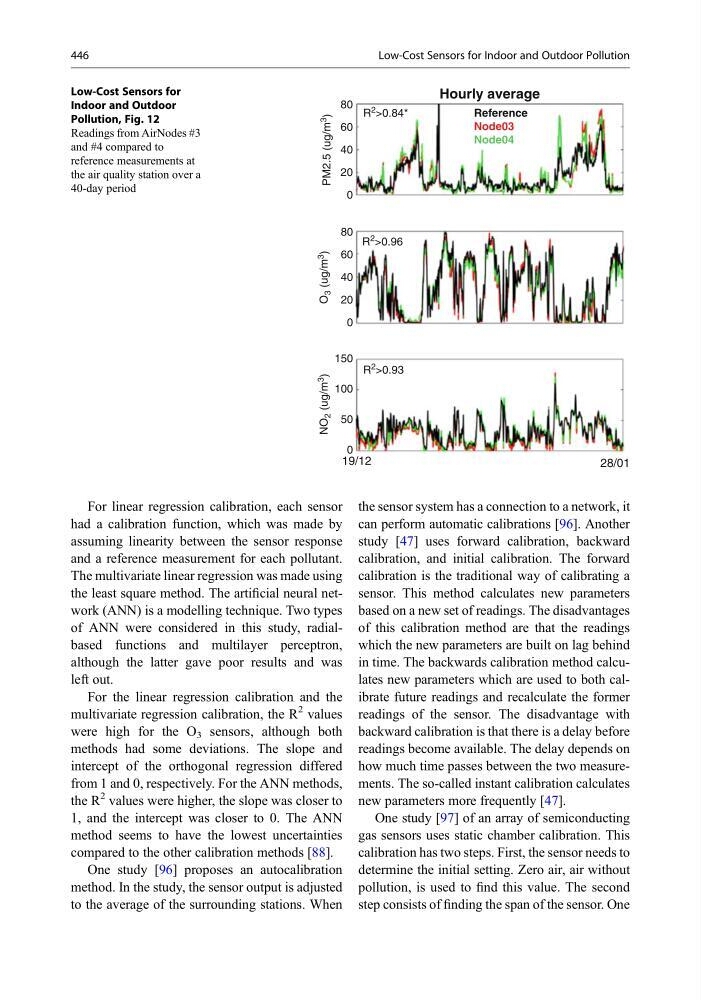
Low-Cost Sensors for
Indoor and Outdoor
Pollution, Fig. 12
Readings from AirNodes #3
and #4 compared to
reference measurements at
the air quality station over a
40-day period
446
Low-Cost Sensors for Indoor and Outdoor Pollution
had a calibration function, which was made by
assuming linearity between the sensor response
and a reference measurement for each pollutant.
The multivariate linear regression was made using
the least square method. The artificial neural network (ANN) is a modelling technique. Two types
of ANN were considered in this study, radialbased functions and multilayer perceptron,
although the latter gave poor results and was
left out.
For the linear regression calibration and the
multivariate regression calibration, the R
2 values
were high for the O 3 sensors, although both
methods had some deviations. The slope and
intercept of the orthogonal regression differed
from 1 and 0, respectively. For the ANN methods,
the R
2 values were higher, the slope was closer to
1, and the intercept was closer to 0. The ANN
method seems to have the lowest uncertainties
compared to the other calibration methods [88].
One study [96] proposes an autocalibration
method. In the study, the sensor output is adjusted
to the average of the surrounding stations. When
the sensor system has a connection to a network, it
can perform automatic calibrations [96]. Another
study [47] uses forward calibration, backward
calibration, and initial calibration. The forward
calibration is the traditional way of calibrating a
sensor. This method calculates new parameters
based on a new set of readings. The disadvantages
of this calibration method are that the readings
which the new parameters are built on lag behind
in time. The backwards calibration method calculates new parameters which are used to both calibrate future readings and recalculate the former
readings of the sensor. The disadvantage with
backward calibration is that there is a delay before
readings become available. The delay depends on
how much time passes between the two measurements. The so-called instant calibration calculates
new parameters more frequently [47].
One study [97] of an array of semiconducting
gas sensors uses static chamber calibration. This
calibration has two steps. First, the sensor needs to
determine the initial setting. Zero air, air without
pollution, is used to find this value. The second
step consists of finding the span of the sensor. One
Hourly average
R 2 >0.84*
R
2 >0.96
R
2 >0.93
PM2.5 (ug/m
3
)
O
3 (ug/m
3
)
NO
2 (ug/m
3
)
80
60
40
20
0
80
60
40
20
0
150
100
50
0
19/12
28/01
Reference
Node03
Node04
Low-Cost Sensors for
Indoor and Outdoor
Pollution, Fig. 12
Readings from AirNodes #3
and #4 compared to
reference measurements at
the air quality station over a
40-day period
446
Low-Cost Sensors for Indoor and Outdoor Pollution