

building, a regular building array, and a complex
urban junction. The examples mainly comprise
simulations using an FCM (specifically a CFD
model); one example using an FAM is also
presented.
CFD models do not describe all meteorological
phenomena as described earlier; however, they are
useful tools for predicting flow characteristics in
street canyons and within urban areas at the neighborhood, building, and street scale. They can also
be used to interpret wind tunnel and field data and
their outputs can therefore be used to improve
operational models. Most available general purpose CFD models currently still need to be validated against wind tunnel or field data to obtain
confidence before applying them to a particular
case study [67]. Some FAM models used for calculating dispersion at the building and street scale
are reviewed in [68].
Single Building
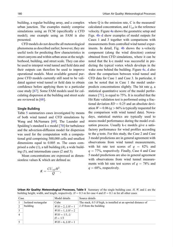
Table 5 summarizes cases investigated by means
of both wind tunnel and CFD simulations by
Wang and McNamara [69]. The Launder and
Spalding’s standard k-ε model [70] for turbulence
and the advection-diffusion model for dispersion
was used for the computation with a computational grid comprising 500,000 cells and smallest
dimensions equal to 0.005 m. The cases comprised a cube (1), a tall building (4), a wide building (5), and intermediate cases (2 and 3).
Mean concentrations are expressed as dimensionless values K which are defined as:
K ¼
CU ref H
2
Q
,
where Q is the emission rate, C is the measured/
calculated concentration, and U ref is the reference
velocity. Figure 4a shows the geometric setup and
Figs. 4b–d show examples of model outputs for
Cases 1 and 3 together with comparisons with
measurements from controlled wind tunnel experiments. In detail, Fig. 4b shows the x-velocity
component (along the wind direction) contour
obtained from CFD simulations, where it can be
noted that the k-ε model was successful in predicting the typical vortex which develops in the
wake zone behind the building. Figure 4c, d also
show the comparison between wind tunnel and
CFD data for Case 1 and Case 3. In particular, it
can be noted that in Case 1 the model underpredicts concentrations slightly. The hit rate q, a
statistical quantitative score of the model performance [71], is equal to 75%. It is recalled that the
Hit Rate validation test is performed using a fractional deviation RD ¼ 0.25 and an absolute deviation W ¼ 0.06 (q > 66% is typically requested for
the comparison with wind tunnel data). Nowadays, statistical metrics are typically used to
assess model performance during the model evaluation process. Usually k-ε models give a satisfactory performance for wind profiles according
to the q tests. For this study, the Case 2 and Case
3 model predictions are in general agreement with
observations from wind tunnel measurements,
with hit rate test scores of q ¼ 82% and
q ¼ 77%, respectively. Finally, Case 4 and Case
5 model predictions are also in general agreement
with observations from wind tunnel measurements with hit rate test scores of q ¼ 78% and
q ¼ 68%, respectively.
Urban Air Quality: Meteorological Processes, Table 5 Summary of the single building case. H, W, and L are the
building height, width, and length, respectively. H ¼ 0.3 m for case 4 and H ¼ 0.1 m for all other cases
Case
Model details
Source details
1 Isolated rectangular
building
Cube
The stack, 0.5 H high, is installed at an upwind distance of
2 H from the building
2
W/H ¼ 2, L/H ¼ 1
3
W/H ¼ 1, L/H ¼ 2
4
W/H ¼ 1/3, L/
H ¼ 1/3
5
W/H ¼ 6, L/H ¼ 1
180
Urban Air Quality: Meteorological Processes
urban junction. The examples mainly comprise
simulations using an FCM (specifically a CFD
model); one example using an FAM is also
presented.
CFD models do not describe all meteorological
phenomena as described earlier; however, they are
useful tools for predicting flow characteristics in
street canyons and within urban areas at the neighborhood, building, and street scale. They can also
be used to interpret wind tunnel and field data and
their outputs can therefore be used to improve
operational models. Most available general purpose CFD models currently still need to be validated against wind tunnel or field data to obtain
confidence before applying them to a particular
case study [67]. Some FAM models used for calculating dispersion at the building and street scale
are reviewed in [68].
Single Building
Table 5 summarizes cases investigated by means
of both wind tunnel and CFD simulations by
Wang and McNamara [69]. The Launder and
Spalding’s standard k-ε model [70] for turbulence
and the advection-diffusion model for dispersion
was used for the computation with a computational grid comprising 500,000 cells and smallest
dimensions equal to 0.005 m. The cases comprised a cube (1), a tall building (4), a wide building (5), and intermediate cases (2 and 3).
Mean concentrations are expressed as dimensionless values K which are defined as:
K ¼
CU ref H
2
Q
,
where Q is the emission rate, C is the measured/
calculated concentration, and U ref is the reference
velocity. Figure 4a shows the geometric setup and
Figs. 4b–d show examples of model outputs for
Cases 1 and 3 together with comparisons with
measurements from controlled wind tunnel experiments. In detail, Fig. 4b shows the x-velocity
component (along the wind direction) contour
obtained from CFD simulations, where it can be
noted that the k-ε model was successful in predicting the typical vortex which develops in the
wake zone behind the building. Figure 4c, d also
show the comparison between wind tunnel and
CFD data for Case 1 and Case 3. In particular, it
can be noted that in Case 1 the model underpredicts concentrations slightly. The hit rate q, a
statistical quantitative score of the model performance [71], is equal to 75%. It is recalled that the
Hit Rate validation test is performed using a fractional deviation RD ¼ 0.25 and an absolute deviation W ¼ 0.06 (q > 66% is typically requested for
the comparison with wind tunnel data). Nowadays, statistical metrics are typically used to
assess model performance during the model evaluation process. Usually k-ε models give a satisfactory performance for wind profiles according
to the q tests. For this study, the Case 2 and Case
3 model predictions are in general agreement with
observations from wind tunnel measurements,
with hit rate test scores of q ¼ 82% and
q ¼ 77%, respectively. Finally, Case 4 and Case
5 model predictions are also in general agreement
with observations from wind tunnel measurements with hit rate test scores of q ¼ 78% and
q ¼ 68%, respectively.
Urban Air Quality: Meteorological Processes, Table 5 Summary of the single building case. H, W, and L are the
building height, width, and length, respectively. H ¼ 0.3 m for case 4 and H ¼ 0.1 m for all other cases
Case
Model details
Source details
1 Isolated rectangular
building
Cube
The stack, 0.5 H high, is installed at an upwind distance of
2 H from the building
2
W/H ¼ 2, L/H ¼ 1
3
W/H ¼ 1, L/H ¼ 2
4
W/H ¼ 1/3, L/
H ¼ 1/3
5
W/H ¼ 6, L/H ¼ 1
180
Urban Air Quality: Meteorological Processes