

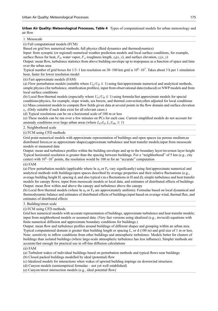
Urban Air Quality: Meteorological Processes, Table 4 Types of computational models for urban meteorology and
air flow
1. Mesoscale
(i) Full computational models (FCM)
Based on grid box numerical methods; full physics (fluid dynamics and thermodynamics)
Input: from synoptic (or regional) numerical weather prediction models and local surface conditions, for example,
surface fluxes for heat, F θ , water vapor, F v , roughness length, z 0 (x, y), and surface elevation, z s (x, y)
Output: mean flow, turbulence statistics from above building envelope up to tropopause as a function of space and time
over the urban area
Typical number of grid boxes for 1/3–1 km resolution on 30–100 km grid is 10
6
–10
7
. Takes about 3 h per 1 simulation
hour, faster for lower resolution model
(ii) Fast approximate models (FAM)
(a) Flow perturbation models (suitable where U G /U B ≳ 1) using fast/approximate numerical and analytical methods,
simple physics (for turbulence, stratification profiles), input from observational data (reduced) or NWP models and from
local surface conditions
(b) Local flow/thermal models (especially where U G /U B ≲ 1) using formula/fast approximate models for special
conditions/physics, for example, slope winds, sea breeze, and thermal convection;often adjusted for local conditions
(c) Mass consistent models to compute flow fields given data at several points in the flow domain and surface elevation
z s . (Only suitable if such data exist for all relevant cases.)
(d) Typical resolutions can be on a horizontal scale of 100 m or less
(e) These models can be run over a few minutes on PCs for each case. Current simplified models do not account for
unsteady conditions over large urban areas (where L O /L f , L c /L Ro ≳ 1)
2. Neighborhood scale
(i) FCM using CFD methods
Grid point numerical models with approximate representation of buildings and open spaces (as porous medium;as
distributed forces;or as approximate shapes);approximate turbulence and heat transfer models;input from mesoscale
models or measured data
Output: mean and turbulence profiles within the building envelope and up to the boundary layer/inversion layer height
Typical horizontal resolution is greater than the spacing between buildings. For a “neighborhood” of 5 km (e.g., city
center) with 10
6
–10
7 points, the resolution would be 100 m for an “accurate” computation
(ii) FAM
(a) Flow perturbation models (applicable where ln z 0 or F θ vary significantly) using fast/approximate numerical and
analytical methods with buildings/open spaces described by average properties and their relative fluctuations (e.g.,
average building height H, spacing d, and also typical r.m.s fluctuations in H and d); simple turbulence and heat transfer
models for canopy flows; input from mesoscale models or local data, and estimates of distributed effects of buildings
Output: mean flow within and above the canopy and turbulence above the canopy
(b) Local flow/thermal models (where ln z 0 or F θ are approximately uniform). Formulae based on local dynamical and
thermodynamic balance and estimates of distributed effects of buildings;input based on average wind, thermal flux, and
estimates of distributed effects
3. Building/street scale
(i) FCM using CFD methods
Grid box numerical models with accurate representation of buildings, approximate turbulence and heat transfer models;
input from neighborhood models or assumed data. (Very fast versions using idealized (e.g., inviscid) equations with
finite numerical diffusion and approximate boundary conditions for buildings.)
Output: mean flow and turbulence profiles around buildings of different shapes and grouping within an urban area.
Typical computational domain is greater than building length or spacing L, or d (100 m) and grid size of 1 m or less.
Note: sensitivity to inflow conditions from other buildings and atmospheric turbulence. Models better for clusters of
buildings than isolated buildings (where large-scale atmospheric turbulence has less influence). Simpler methods are
accurate/fast enough for practical use in off-line diffusion calculations
(ii) FAM
(a) Turbulent wakes of individual buildings based on perturbation methods and typical flows near buildings
(b) Closed packed buildings modelled by ideal (potential) flow
(c) Idealized models for interactions when wakes of upwind building impinge on downwind structures
(d) Canyon models (semiempirical formulae – not yet well established)
(e) Canyon/street intersection models (e.g., ideal potential flow)
Urban Air Quality: Meteorological Processes
175
air flow
1. Mesoscale
(i) Full computational models (FCM)
Based on grid box numerical methods; full physics (fluid dynamics and thermodynamics)
Input: from synoptic (or regional) numerical weather prediction models and local surface conditions, for example,
surface fluxes for heat, F θ , water vapor, F v , roughness length, z 0 (x, y), and surface elevation, z s (x, y)
Output: mean flow, turbulence statistics from above building envelope up to tropopause as a function of space and time
over the urban area
Typical number of grid boxes for 1/3–1 km resolution on 30–100 km grid is 10
6
–10
7
. Takes about 3 h per 1 simulation
hour, faster for lower resolution model
(ii) Fast approximate models (FAM)
(a) Flow perturbation models (suitable where U G /U B ≳ 1) using fast/approximate numerical and analytical methods,
simple physics (for turbulence, stratification profiles), input from observational data (reduced) or NWP models and from
local surface conditions
(b) Local flow/thermal models (especially where U G /U B ≲ 1) using formula/fast approximate models for special
conditions/physics, for example, slope winds, sea breeze, and thermal convection;often adjusted for local conditions
(c) Mass consistent models to compute flow fields given data at several points in the flow domain and surface elevation
z s . (Only suitable if such data exist for all relevant cases.)
(d) Typical resolutions can be on a horizontal scale of 100 m or less
(e) These models can be run over a few minutes on PCs for each case. Current simplified models do not account for
unsteady conditions over large urban areas (where L O /L f , L c /L Ro ≳ 1)
2. Neighborhood scale
(i) FCM using CFD methods
Grid point numerical models with approximate representation of buildings and open spaces (as porous medium;as
distributed forces;or as approximate shapes);approximate turbulence and heat transfer models;input from mesoscale
models or measured data
Output: mean and turbulence profiles within the building envelope and up to the boundary layer/inversion layer height
Typical horizontal resolution is greater than the spacing between buildings. For a “neighborhood” of 5 km (e.g., city
center) with 10
6
–10
7 points, the resolution would be 100 m for an “accurate” computation
(ii) FAM
(a) Flow perturbation models (applicable where ln z 0 or F θ vary significantly) using fast/approximate numerical and
analytical methods with buildings/open spaces described by average properties and their relative fluctuations (e.g.,
average building height H, spacing d, and also typical r.m.s fluctuations in H and d); simple turbulence and heat transfer
models for canopy flows; input from mesoscale models or local data, and estimates of distributed effects of buildings
Output: mean flow within and above the canopy and turbulence above the canopy
(b) Local flow/thermal models (where ln z 0 or F θ are approximately uniform). Formulae based on local dynamical and
thermodynamic balance and estimates of distributed effects of buildings;input based on average wind, thermal flux, and
estimates of distributed effects
3. Building/street scale
(i) FCM using CFD methods
Grid box numerical models with accurate representation of buildings, approximate turbulence and heat transfer models;
input from neighborhood models or assumed data. (Very fast versions using idealized (e.g., inviscid) equations with
finite numerical diffusion and approximate boundary conditions for buildings.)
Output: mean flow and turbulence profiles around buildings of different shapes and grouping within an urban area.
Typical computational domain is greater than building length or spacing L, or d (100 m) and grid size of 1 m or less.
Note: sensitivity to inflow conditions from other buildings and atmospheric turbulence. Models better for clusters of
buildings than isolated buildings (where large-scale atmospheric turbulence has less influence). Simpler methods are
accurate/fast enough for practical use in off-line diffusion calculations
(ii) FAM
(a) Turbulent wakes of individual buildings based on perturbation methods and typical flows near buildings
(b) Closed packed buildings modelled by ideal (potential) flow
(c) Idealized models for interactions when wakes of upwind building impinge on downwind structures
(d) Canyon models (semiempirical formulae – not yet well established)
(e) Canyon/street intersection models (e.g., ideal potential flow)
Urban Air Quality: Meteorological Processes
175