

24 unifying physics of accelerators, lasers and plasma
2.3 Equations of motion
2.3.1 Motion of charged particles in EM fields
The motion of a particle with charge q in an electric E and
magnetic B fields is given by the following equations:
dp
d
= q(E + v
E
× B) ,
= F · v
(2.10)
dt
dt
where the momentum p and energy E of the particle are
p = m 0 γv , E =
2
m 0 γc
and m 0 is the particle mass, and γ is the relativistic factor.
Let’s consider the case of the uniform magnetic field when
the equation of motion simplifies to
dγv
m 0
= qv × B or m 0 γ v˙ x = q v y B and m 0 γ v˙ y = −q v x B
dt
which then can be rewritten as
2
qB
qB
v ¨ x =
v˙ y =
0 γ
−
(
v x
m
m 0 γ
)
which has a solution of
v
v x =
0
v 0 cos(ωt) or x =
sin(ωt)
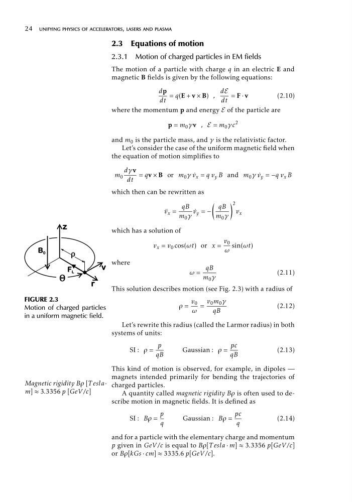
FIGURE 2.3
Motion of charged particles
in a uniform magnetic field.
T
s
ω
where
qB
ω =
(2.11)
m 0 γ
his solution describes motion (see Fig. 2.3) with a radius of
v 0 v 0 m
=
=
0 γ
ρ
(2.12)
ω
qB
Let’s rewrite this radius (called the Larmor radius) in both
ystems of units:
p
pc
SI : ρ =
Gaussian : ρ =
(2.13)
qB
qB
This kind of motion is observed, for example, in dipoles —
magnets intended primarily for bending the trajectories of
Magnetic rigidity Bρ [T esla · charged particles.
m] ≈ 3.3356 p [GeV /c]
A quantity called magnetic rigidity Bρ is often used to describe motion in magnetic fields. It is defined as
p
pc
SI : Bρ =
Gaussian : Bρ =
(2.14)
q
q
and for a particle with the elementary charge and momentum
p given in GeV /c is equal to Bρ[T esla · m] ≈ 3.3356 p[GeV /c]
or Bρ[kGs · cm] ≈ 3335.6 p[GeV /c].
2.3 Equations of motion
2.3.1 Motion of charged particles in EM fields
The motion of a particle with charge q in an electric E and
magnetic B fields is given by the following equations:
dp
d
= q(E + v
E
× B) ,
= F · v
(2.10)
dt
dt
where the momentum p and energy E of the particle are
p = m 0 γv , E =
2
m 0 γc
and m 0 is the particle mass, and γ is the relativistic factor.
Let’s consider the case of the uniform magnetic field when
the equation of motion simplifies to
dγv
m 0
= qv × B or m 0 γ v˙ x = q v y B and m 0 γ v˙ y = −q v x B
dt
which then can be rewritten as
2
qB
qB
v ¨ x =
v˙ y =
0 γ
−
(
v x
m
m 0 γ
)
which has a solution of
v
v x =
0
v 0 cos(ωt) or x =
sin(ωt)
FIGURE 2.3
Motion of charged particles
in a uniform magnetic field.
T
s
ω
where
qB
ω =
(2.11)
m 0 γ
his solution describes motion (see Fig. 2.3) with a radius of
v 0 v 0 m
=
=
0 γ
ρ
(2.12)
ω
qB
Let’s rewrite this radius (called the Larmor radius) in both
ystems of units:
p
pc
SI : ρ =
Gaussian : ρ =
(2.13)
qB
qB
This kind of motion is observed, for example, in dipoles —
magnets intended primarily for bending the trajectories of
Magnetic rigidity Bρ [T esla · charged particles.
m] ≈ 3.3356 p [GeV /c]
A quantity called magnetic rigidity Bρ is often used to describe motion in magnetic fields. It is defined as
p
pc
SI : Bρ =
Gaussian : Bρ =
(2.14)
q
q
and for a particle with the elementary charge and momentum
p given in GeV /c is equal to Bρ[T esla · m] ≈ 3.3356 p[GeV /c]
or Bρ[kGs · cm] ≈ 3335.6 p[GeV /c].