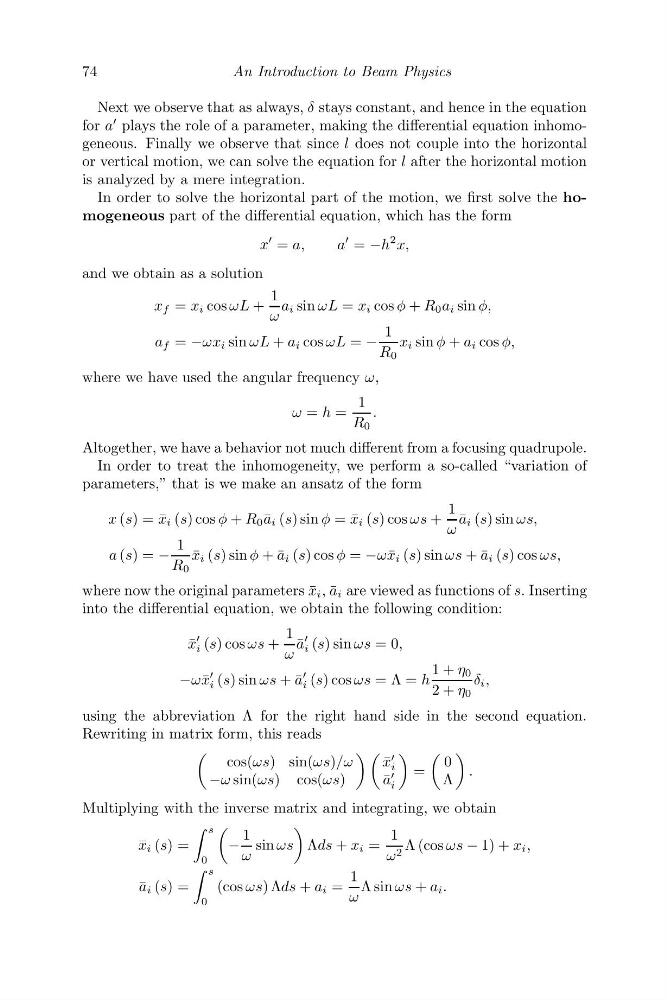
74
An Introduction to Beam Physics
Next we observe that as always, δ stays constant, and hence in the equation
for a
plays the role of a parameter, making the differential equation inhomogeneous. Finally we observe that since l does not couple into the horizontal
or vertical motion, we can solve the equation for l after the horizontal motion
is analyzed by a mere integration.
In order to solve the horizontal part of the motion, we first solve the homogeneous part of the differential equation, which has the form
x
= a,
a
= −h
2 x,
and we obtain as a solution
x f = x i cos ωL +
1
ω
a i sin ωL = x i cos φ + R 0 a i sin φ,
a f = −ωx i sin ωL + a i cos ωL = −
1
R 0
x i sin φ + a i cos φ,
where we have used the angular frequency ω,
ω = h =
1
R 0
.
Altogether, we have a behavior not much different from a focusing quadrupole.
In order to treat the inhomogeneity, we perform a so-called “variation of
parameters,” that is we make an ansatz of the form
x (s) = ¯
x i (s) cos φ + R 0 ¯
a i (s) sin φ = ¯
x i (s) cos ωs +
1
ω
¯
a i (s) sin ωs,
a (s) = −
1
R 0
¯
x i (s) sin φ + ¯
a i (s) cos φ = −ω ¯
x i (s) sin ωs + ¯
a i (s) cos ωs,
where now the original parameters ¯
x i , ¯
a i are viewed as functions of s. Inserting
into the differential equation, we obtain the following condition:
¯
x
i (s) cos ωs +
1
ω
¯
a
i (s) sin ωs = 0,
−ω ¯
x
i (s) sin ωs + ¯
a
i (s) cos ωs = Λ = h
1 + η 0
2 + η 0
δ i ,
using the abbreviation Λ for the right hand side in the second equation.
Rewriting in matrix form, this reads
cos(ωs) sin(ωs)/ω
−ω sin(ωs) cos(ωs)
¯
x
i
¯
a
i
=
0
Λ
.
Multiplying with the inverse matrix and integrating, we obtain
¯
x i (s) =
s
0
−
1
ω
sin ωs
Λds + x i =
1
ω 2 Λ (cos ωs − 1) + x i ,
¯
a i (s) =
s
0
(cos ωs) Λds + a i =
1
ω
Λ sin ωs + a i .