

52
An Introduction to Beam Physics
By induction over k, we now show that M k,l = 0 for all cases where k < l.
Apparently the statement is true for k = 0 as we just showed. Now let us
assume that the statement is true up to k − 1. If k < l, also k − 2 < l, and thus
M
k−2,l (s) = 0. Since k
2
− l
2
= 0 and cos (lφ + θ k,l ) = 0 for some φ because
l = 0, this requires
M k,l (s) = 0 for k < l.
Thus the infinite matrix M k,l is strictly lower triangular.
We now study the situation for different values of l. We first notice that for
all l, the choices of
M l,l (s) and θ l,l are free
because M
l−2,l (s) = 0 by the previous observation, and k
2
− l
2 = 0 for k = l.
Next we observe that the value M l+1,l (s) must vanish, because k
2
− l
2
= 0,
but M
l−1,l (s) = 0 because of the lower triangularity. Recursively we even
obtain that
M l+1,l (s), M l+3,l (s), . . . vanish.
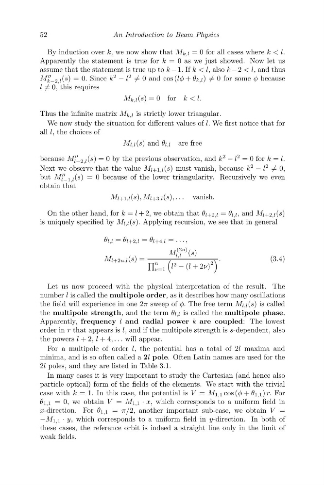
On the other hand, for k = l + 2, we obtain that θ l+2,l = θ l,l , and M l+2,l (s)
is uniquely specified by M l,l (s). Applying recursion, we see that in general
θ l,l = θ l+2,l = θ l+4,l = . . . ,
M l+2n,l (s) =
M
(2n)
l,l (s)
n
ν=1
l 2 − (l + 2ν)
2
.
(3.4)
Let us now proceed with the physical interpretation of the result. The
number l is called the multipole order, as it describes how many oscillations
the field will experience in one 2π sweep of φ. The free term M l,l (s) is called
the multipole strength, and the term θ l,l is called the multipole phase.
Apparently, frequency l and radial power k are coupled: The lowest
order in r that appears is l, and if the multipole strength is s-dependent, also
the powers l + 2, l + 4, . . . will appear.
For a multipole of order l, the potential has a total of 2l maxima and
minima, and is so often called a 2l pole. Often Latin names are used for the
2l poles, and they are listed in Table 3.1.
In many cases it is very important to study the Cartesian (and hence also
particle optical) form of the fields of the elements. We start with the trivial
case with k = 1. In this case, the potential is V = M 1,1 cos (φ + θ 1,1 ) r. For
θ 1,1 = 0, we obtain V = M 1,1 · x, which corresponds to a uniform field in
x-direction. For θ 1,1 = π/2, another important sub-case, we obtain V =
−M 1,1 · y, which corresponds to a uniform field in y-direction. In both of
these cases, the reference orbit is indeed a straight line only in the limit of
weak fields.
An Introduction to Beam Physics
By induction over k, we now show that M k,l = 0 for all cases where k < l.
Apparently the statement is true for k = 0 as we just showed. Now let us
assume that the statement is true up to k − 1. If k < l, also k − 2 < l, and thus
M
k−2,l (s) = 0. Since k
2
− l
2
= 0 and cos (lφ + θ k,l ) = 0 for some φ because
l = 0, this requires
M k,l (s) = 0 for k < l.
Thus the infinite matrix M k,l is strictly lower triangular.
We now study the situation for different values of l. We first notice that for
all l, the choices of
M l,l (s) and θ l,l are free
because M
l−2,l (s) = 0 by the previous observation, and k
2
− l
2 = 0 for k = l.
Next we observe that the value M l+1,l (s) must vanish, because k
2
− l
2
= 0,
but M
l−1,l (s) = 0 because of the lower triangularity. Recursively we even
obtain that
M l+1,l (s), M l+3,l (s), . . . vanish.
On the other hand, for k = l + 2, we obtain that θ l+2,l = θ l,l , and M l+2,l (s)
is uniquely specified by M l,l (s). Applying recursion, we see that in general
θ l,l = θ l+2,l = θ l+4,l = . . . ,
M l+2n,l (s) =
M
(2n)
l,l (s)
n
ν=1
l 2 − (l + 2ν)
2
.
(3.4)
Let us now proceed with the physical interpretation of the result. The
number l is called the multipole order, as it describes how many oscillations
the field will experience in one 2π sweep of φ. The free term M l,l (s) is called
the multipole strength, and the term θ l,l is called the multipole phase.
Apparently, frequency l and radial power k are coupled: The lowest
order in r that appears is l, and if the multipole strength is s-dependent, also
the powers l + 2, l + 4, . . . will appear.
For a multipole of order l, the potential has a total of 2l maxima and
minima, and is so often called a 2l pole. Often Latin names are used for the
2l poles, and they are listed in Table 3.1.
In many cases it is very important to study the Cartesian (and hence also
particle optical) form of the fields of the elements. We start with the trivial
case with k = 1. In this case, the potential is V = M 1,1 cos (φ + θ 1,1 ) r. For
θ 1,1 = 0, we obtain V = M 1,1 · x, which corresponds to a uniform field in
x-direction. For θ 1,1 = π/2, another important sub-case, we obtain V =
−M 1,1 · y, which corresponds to a uniform field in y-direction. In both of
these cases, the reference orbit is indeed a straight line only in the limit of
weak fields.