

50
An Introduction to Beam Physics
In order to study the solutions of Laplace’s equations for the electric and
magnetic scalar potentials, we will proceed for two special cases, each of which
will be treated in a coordinate system most suitable for the problem.
3.1 Fields with Straight Reference Orbit
The first major case of systems is those that have a straight reference orbit.
In this case, there is no need to distinguish between particle optical coordinates
and Cartesian coordinates, and in particular there is no need to transform
Laplace’s equation to a new set of coordinates. Many elements with a straight
reference orbit possess a certain rotational symmetry around the axis of
the reference orbit, and it is most advantageous to describe the potential in
cylindrical coordinates with a longitudinal z-axis that coincides with the
reference orbit.
3.1.1 Expansion in Cylindrical Coordinates
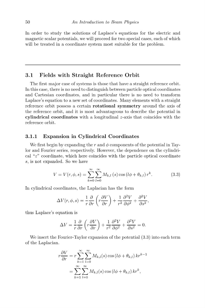
We first begin by expanding the r and φ components of the potential in Taylor and Fourier series, respectively. However, the dependence on the cylindrical “z” coordinate, which here coincides with the particle optical coordinate
s, is not expanded. So we have
V = V (r, φ, s) =
∞
k=0
∞
l=0
M k,l (s) cos (lφ + θ k,l ) r
k .
(3.3)
In cylindrical coordinates, the Laplacian has the form
ΔV (r, φ, s) =
1
r
∂
∂r
r
∂V
∂r
+
1
r 2
∂
2 V
∂φ 2 +
∂
2 V
∂s 2 ,
thus Laplace’s equation is
ΔV =
1
r
∂
∂r
r
∂V
∂r
+
1
r 2
∂
2 V
∂φ 2 +
∂
2 V
∂s 2 = 0.
We insert the Fourier-Taylor expansion of the potential (3.3) into each term
of the Laplacian.
r
∂V
∂r
= r
∞
k=1
∞
l=0
M k,l (s) cos (lφ + θ k,l ) kr
k−1
=
∞
k=1
∞
l=0
M k,l (s) cos (lφ + θ k,l ) kr
k ,
An Introduction to Beam Physics
In order to study the solutions of Laplace’s equations for the electric and
magnetic scalar potentials, we will proceed for two special cases, each of which
will be treated in a coordinate system most suitable for the problem.
3.1 Fields with Straight Reference Orbit
The first major case of systems is those that have a straight reference orbit.
In this case, there is no need to distinguish between particle optical coordinates
and Cartesian coordinates, and in particular there is no need to transform
Laplace’s equation to a new set of coordinates. Many elements with a straight
reference orbit possess a certain rotational symmetry around the axis of
the reference orbit, and it is most advantageous to describe the potential in
cylindrical coordinates with a longitudinal z-axis that coincides with the
reference orbit.
3.1.1 Expansion in Cylindrical Coordinates
We first begin by expanding the r and φ components of the potential in Taylor and Fourier series, respectively. However, the dependence on the cylindrical “z” coordinate, which here coincides with the particle optical coordinate
s, is not expanded. So we have
V = V (r, φ, s) =
∞
k=0
∞
l=0
M k,l (s) cos (lφ + θ k,l ) r
k .
(3.3)
In cylindrical coordinates, the Laplacian has the form
ΔV (r, φ, s) =
1
r
∂
∂r
r
∂V
∂r
+
1
r 2
∂
2 V
∂φ 2 +
∂
2 V
∂s 2 ,
thus Laplace’s equation is
ΔV =
1
r
∂
∂r
r
∂V
∂r
+
1
r 2
∂
2 V
∂φ 2 +
∂
2 V
∂s 2 = 0.
We insert the Fourier-Taylor expansion of the potential (3.3) into each term
of the Laplacian.
r
∂V
∂r
= r
∞
k=1
∞
l=0
M k,l (s) cos (lφ + θ k,l ) kr
k−1
=
∞
k=1
∞
l=0
M k,l (s) cos (lφ + θ k,l ) kr
k ,