

Linear Beam Optics
35
In light of this, the entire action of a beam physics device can now be
expressed by how it manipulates the coordinates in
Z. In fact, usually a set of
initial conditions
Z 0 at position s 0 uniquely determines the future evolution
and hence
Z at any later position s. While a common notion, mathematically
this determinism of classical mechanics rests on some subtle assumptions
about the details of the fields that are allowed in the motion; but further
details are beyond this book.
Assuming that indeed
Z 0 at s 0 uniquely determines the future evolution,
we can define a function relating the initial conditions at s 0 to the conditions
at s via
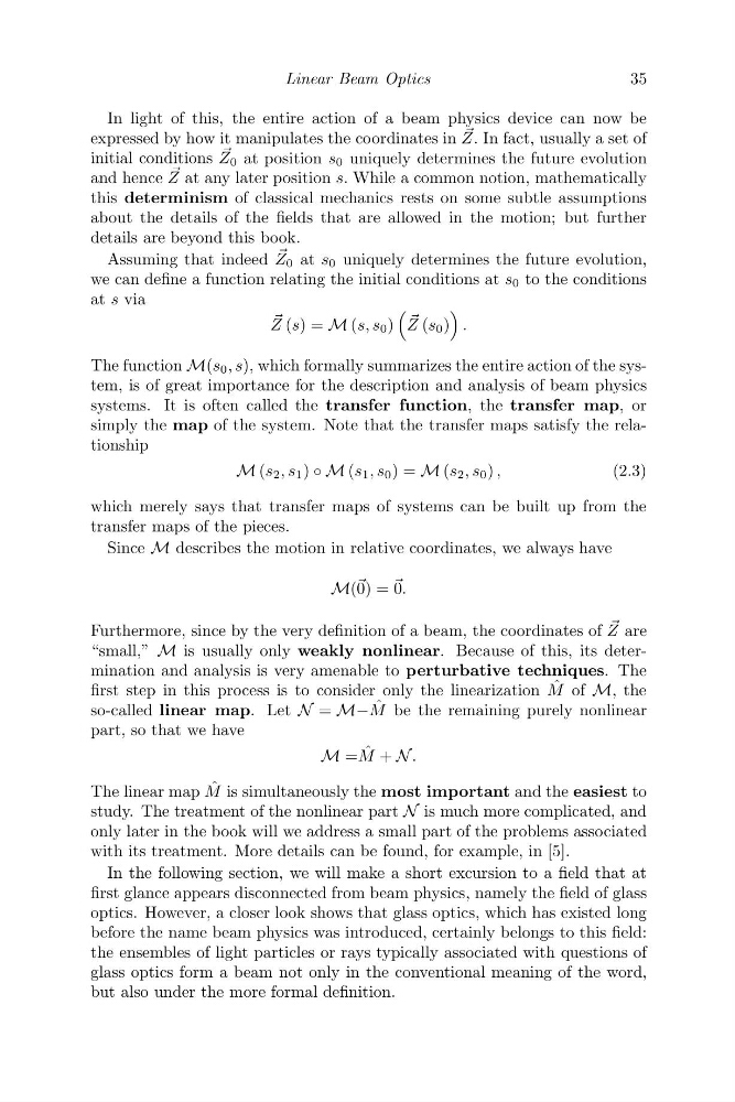
Z (s) = M (s, s 0 )
Z (s 0 )
.
The function M(s 0 , s), which formally summarizes the entire action of the system, is of great importance for the description and analysis of beam physics
systems. It is often called the transfer function, the transfer map, or
simply the map of the system. Note that the transfer maps satisfy the relationship
M (s 2 , s 1 ) ◦ M (s 1 , s 0 ) = M (s 2 , s 0 ) ,
(2.3)
which merely says that transfer maps of systems can be built up from the
transfer maps of the pieces.
Since M describes the motion in relative coordinates, we always have
M( 0) = 0.
Furthermore, since by the very definition of a beam, the coordinates of
Z are
“small,” M is usually only weakly nonlinear. Because of this, its determination and analysis is very amenable to perturbative techniques. The
first step in this process is to consider only the linearization ˆ
M of M, the
so-called linear map. Let N = M− ˆ
M be the remaining purely nonlinear
part, so that we have
M = ˆ
M + N .
The linear map ˆ
M is simultaneously the most important and the easiest to
study. The treatment of the nonlinear part N is much more complicated, and
only later in the book will we address a small part of the problems associated
with its treatment. More details can be found, for example, in [5].
In the following section, we will make a short excursion to a field that at
first glance appears disconnected from beam physics, namely the field of glass
optics. However, a closer look shows that glass optics, which has existed long
before the name beam physics was introduced, certainly belongs to this field:
the ensembles of light particles or rays typically associated with questions of
glass optics form a beam not only in the conventional meaning of the word,
but also under the more formal definition.
35
In light of this, the entire action of a beam physics device can now be
expressed by how it manipulates the coordinates in
Z. In fact, usually a set of
initial conditions
Z 0 at position s 0 uniquely determines the future evolution
and hence
Z at any later position s. While a common notion, mathematically
this determinism of classical mechanics rests on some subtle assumptions
about the details of the fields that are allowed in the motion; but further
details are beyond this book.
Assuming that indeed
Z 0 at s 0 uniquely determines the future evolution,
we can define a function relating the initial conditions at s 0 to the conditions
at s via
Z (s) = M (s, s 0 )
Z (s 0 )
.
The function M(s 0 , s), which formally summarizes the entire action of the system, is of great importance for the description and analysis of beam physics
systems. It is often called the transfer function, the transfer map, or
simply the map of the system. Note that the transfer maps satisfy the relationship
M (s 2 , s 1 ) ◦ M (s 1 , s 0 ) = M (s 2 , s 0 ) ,
(2.3)
which merely says that transfer maps of systems can be built up from the
transfer maps of the pieces.
Since M describes the motion in relative coordinates, we always have
M( 0) = 0.
Furthermore, since by the very definition of a beam, the coordinates of
Z are
“small,” M is usually only weakly nonlinear. Because of this, its determination and analysis is very amenable to perturbative techniques. The
first step in this process is to consider only the linearization ˆ
M of M, the
so-called linear map. Let N = M− ˆ
M be the remaining purely nonlinear
part, so that we have
M = ˆ
M + N .
The linear map ˆ
M is simultaneously the most important and the easiest to
study. The treatment of the nonlinear part N is much more complicated, and
only later in the book will we address a small part of the problems associated
with its treatment. More details can be found, for example, in [5].
In the following section, we will make a short excursion to a field that at
first glance appears disconnected from beam physics, namely the field of glass
optics. However, a closer look shows that glass optics, which has existed long
before the name beam physics was introduced, certainly belongs to this field:
the ensembles of light particles or rays typically associated with questions of
glass optics form a beam not only in the conventional meaning of the word,
but also under the more formal definition.