

204
An Introduction to Beam Physics
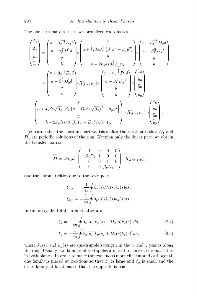
The one turn map in the new normalized coordinates is
⎛
⎜
⎜
⎜
⎜
⎝
x 1
a 1
y 1
b 1
⎞
⎟
⎟
⎟
⎟
⎠
=
⎛
⎜
⎜
⎜
⎜
⎝
x + β
−
1
2
x D x δ
a + β
1
2
x D
x δ
y
b
⎞
⎟
⎟
⎟
⎟
⎠
◦
⎛
⎜
⎜
⎜
⎜
⎝
x
a + k s dsβ
1
2
x
β x x
2
− β y y
2
y
b − 2k s dsβ
1
2
x β y xy
⎞
⎟
⎟
⎟
⎟
⎠
◦
⎛
⎜
⎜
⎜
⎜
⎝
x − β
−
1
2
x D x δ
a − β
1
2
x D
x δ
y
b
⎞
⎟
⎟
⎟
⎟
⎠
◦
⎛
⎜
⎜
⎜
⎜
⎝
x + β
−
1
2
x D x δ
a + β
1
2
x D
x δ
y
b
⎞
⎟
⎟
⎟
⎟
⎠
◦R(μ x , μ y )◦
⎛
⎜
⎜
⎜
⎜
⎝
x − β
−
1
2
x D x δ
a − β
1
2
x D
x δ
y
b
⎞
⎟
⎟
⎟
⎟
⎠
◦
⎛
⎜
⎜
⎜
⎜
⎝
x 0
a 0
y 0
b 0
⎞
⎟
⎟
⎟
⎟
⎠
=
⎛
⎜
⎜
⎜
⎝
x
a + k s ds
√
β x
β x
x − D x δ/
√
β x
2 − β y y
2
y
b − 2k s ds
√
β x β y
x − D x δ/
√
β x
y
⎞
⎟
⎟
⎟
⎠
◦ R(μ x , μ y ) ◦
⎛
⎜
⎜
⎜
⎝
x 0
a 0
y 0
b 0
⎞
⎟
⎟
⎟
⎠
.
The reason that the constant part vanishes after the rotation is that D x and
D
x are periodic solutions of the ring. Keeping only the linear part, we obtain
the transfer matrix
ˆ
M = 2δk s ds
⎛
⎜
⎜
⎝
1
0 0 0
−β x D x 1 0 0
0
0 1 0
0
0 β y D x 1
⎞
⎟
⎟
⎠ · ˆ
R(μ x , μ y ),
and the chromaticities due to the sextupole
ξ x,s =
1
4π
β x (s)D x (s)k s (s)ds,
ξ y,s = −
1
4π
β y (s)D x (s)k s (s)ds.
In summary the total chromaticities are
ξ x = −
1
4π
β x (s) [k x (s) − D x (s)k s (s)] ds,
(8.4)
ξ y = −
1
4π
β y (s) [k y (s) + D x (s)k s (s)] ds,
(8.5)
where k x (s) and k y (s) are quadrupole strength in the x and y planes along
the ring. Usually two families of sextupoles are used to correct chromaticities
in both planes. In order to make the two knobs more efficient and orthogonal,
one family is placed at locations so that β x is large and β y is small and the
other family at locations so that the opposite is true.
An Introduction to Beam Physics
The one turn map in the new normalized coordinates is
⎛
⎜
⎜
⎜
⎜
⎝
x 1
a 1
y 1
b 1
⎞
⎟
⎟
⎟
⎟
⎠
=
⎛
⎜
⎜
⎜
⎜
⎝
x + β
−
1
2
x D x δ
a + β
1
2
x D
x δ
y
b
⎞
⎟
⎟
⎟
⎟
⎠
◦
⎛
⎜
⎜
⎜
⎜
⎝
x
a + k s dsβ
1
2
x
β x x
2
− β y y
2
y
b − 2k s dsβ
1
2
x β y xy
⎞
⎟
⎟
⎟
⎟
⎠
◦
⎛
⎜
⎜
⎜
⎜
⎝
x − β
−
1
2
x D x δ
a − β
1
2
x D
x δ
y
b
⎞
⎟
⎟
⎟
⎟
⎠
◦
⎛
⎜
⎜
⎜
⎜
⎝
x + β
−
1
2
x D x δ
a + β
1
2
x D
x δ
y
b
⎞
⎟
⎟
⎟
⎟
⎠
◦R(μ x , μ y )◦
⎛
⎜
⎜
⎜
⎜
⎝
x − β
−
1
2
x D x δ
a − β
1
2
x D
x δ
y
b
⎞
⎟
⎟
⎟
⎟
⎠
◦
⎛
⎜
⎜
⎜
⎜
⎝
x 0
a 0
y 0
b 0
⎞
⎟
⎟
⎟
⎟
⎠
=
⎛
⎜
⎜
⎜
⎝
x
a + k s ds
√
β x
β x
x − D x δ/
√
β x
2 − β y y
2
y
b − 2k s ds
√
β x β y
x − D x δ/
√
β x
y
⎞
⎟
⎟
⎟
⎠
◦ R(μ x , μ y ) ◦
⎛
⎜
⎜
⎜
⎝
x 0
a 0
y 0
b 0
⎞
⎟
⎟
⎟
⎠
.
The reason that the constant part vanishes after the rotation is that D x and
D
x are periodic solutions of the ring. Keeping only the linear part, we obtain
the transfer matrix
ˆ
M = 2δk s ds
⎛
⎜
⎜
⎝
1
0 0 0
−β x D x 1 0 0
0
0 1 0
0
0 β y D x 1
⎞
⎟
⎟
⎠ · ˆ
R(μ x , μ y ),
and the chromaticities due to the sextupole
ξ x,s =
1
4π
β x (s)D x (s)k s (s)ds,
ξ y,s = −
1
4π
β y (s)D x (s)k s (s)ds.
In summary the total chromaticities are
ξ x = −
1
4π
β x (s) [k x (s) − D x (s)k s (s)] ds,
(8.4)
ξ y = −
1
4π
β y (s) [k y (s) + D x (s)k s (s)] ds,
(8.5)
where k x (s) and k y (s) are quadrupole strength in the x and y planes along
the ring. Usually two families of sextupoles are used to correct chromaticities
in both planes. In order to make the two knobs more efficient and orthogonal,
one family is placed at locations so that β x is large and β y is small and the
other family at locations so that the opposite is true.