

132
An Introduction to Beam Physics
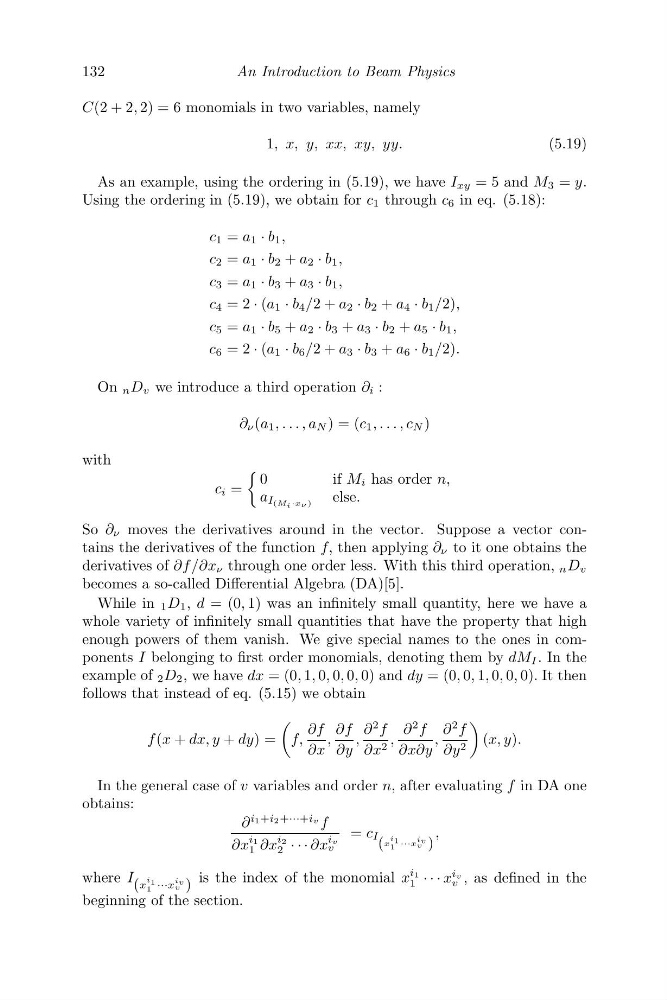
C(2 + 2, 2) = 6 monomials in two variables, namely
1, x, y, xx, xy, yy.
(5.19)
As an example, using the ordering in (5.19), we have I xy = 5 and M 3 = y.
Using the ordering in (5.19), we obtain for c 1 through c 6 in eq. (5.18):
c 1 = a 1 · b 1 ,
c 2 = a 1 · b 2 + a 2 · b 1 ,
c 3 = a 1 · b 3 + a 3 · b 1 ,
c 4 = 2 · (a 1 · b 4 /2 + a 2 · b 2 + a 4 · b 1 /2),
c 5 = a 1 · b 5 + a 2 · b 3 + a 3 · b 2 + a 5 · b 1 ,
c 6 = 2 · (a 1 · b 6 /2 + a 3 · b 3 + a 6 · b 1 /2).
On n D v we introduce a third operation ∂ i :
∂ ν (a 1 , . . . , a N ) = (c 1 , . . . , c N )
with
c i =
0
i fM i has order n,
a I (M i ·xν ) else.
So ∂ ν moves the derivatives around in the vector. Suppose a vector contains the derivatives of the function f, then applying ∂ ν to it one obtains the
derivatives of ∂f /∂x ν through one order less. With this third operation, n D v
becomes a so-called Differential Algebra (DA)[5].
While in 1 D 1 , d = (0, 1) was an infinitely small quantity, here we have a
whole variety of infinitely small quantities that have the property that high
enough powers of them vanish. We give special names to the ones in components I belonging to first order monomials, denoting them by dM I . In the
example of 2 D 2 , we have dx = (0, 1, 0, 0, 0, 0) and dy = (0, 0, 1, 0, 0, 0). It then
follows that instead of eq. (5.15) we obtain
f (x + dx, y + dy) =
f,
∂f
∂x
,
∂f
∂y
,
∂
2 f
∂x 2 ,
∂
2 f
∂x∂y
,
∂
2 f
∂y 2
(x, y).
In the general case of v variables and order n, after evaluating f in DA one
obtains:
∂
i1+i2+···+iv f
∂x
i1
1 ∂x
i2
2 · · · ∂x
iv
v
= c I
( x
i 1
1 ···x
iv
v )
,
where I (x
i 1
1 ···x
iv
v ) is the index of the monomial x
i1
1 · · · x
iv
v , as defined in the
beginning of the section.
An Introduction to Beam Physics
C(2 + 2, 2) = 6 monomials in two variables, namely
1, x, y, xx, xy, yy.
(5.19)
As an example, using the ordering in (5.19), we have I xy = 5 and M 3 = y.
Using the ordering in (5.19), we obtain for c 1 through c 6 in eq. (5.18):
c 1 = a 1 · b 1 ,
c 2 = a 1 · b 2 + a 2 · b 1 ,
c 3 = a 1 · b 3 + a 3 · b 1 ,
c 4 = 2 · (a 1 · b 4 /2 + a 2 · b 2 + a 4 · b 1 /2),
c 5 = a 1 · b 5 + a 2 · b 3 + a 3 · b 2 + a 5 · b 1 ,
c 6 = 2 · (a 1 · b 6 /2 + a 3 · b 3 + a 6 · b 1 /2).
On n D v we introduce a third operation ∂ i :
∂ ν (a 1 , . . . , a N ) = (c 1 , . . . , c N )
with
c i =
0
i fM i has order n,
a I (M i ·xν ) else.
So ∂ ν moves the derivatives around in the vector. Suppose a vector contains the derivatives of the function f, then applying ∂ ν to it one obtains the
derivatives of ∂f /∂x ν through one order less. With this third operation, n D v
becomes a so-called Differential Algebra (DA)[5].
While in 1 D 1 , d = (0, 1) was an infinitely small quantity, here we have a
whole variety of infinitely small quantities that have the property that high
enough powers of them vanish. We give special names to the ones in components I belonging to first order monomials, denoting them by dM I . In the
example of 2 D 2 , we have dx = (0, 1, 0, 0, 0, 0) and dy = (0, 0, 1, 0, 0, 0). It then
follows that instead of eq. (5.15) we obtain
f (x + dx, y + dy) =
f,
∂f
∂x
,
∂f
∂y
,
∂
2 f
∂x 2 ,
∂
2 f
∂x∂y
,
∂
2 f
∂y 2
(x, y).
In the general case of v variables and order n, after evaluating f in DA one
obtains:
∂
i1+i2+···+iv f
∂x
i1
1 ∂x
i2
2 · · · ∂x
iv
v
= c I
( x
i 1
1 ···x
iv
v )
,
where I (x
i 1
1 ···x
iv
v ) is the index of the monomial x
i1
1 · · · x
iv
v , as defined in the
beginning of the section.