

126
An Introduction to Beam Physics
One direct consequence of the symplectic condition and the resulting unity of
the Jacobian determinant is that the volume of the phase space is conserved
under Hamiltonian motion, which is known as Liouville’s theorem.
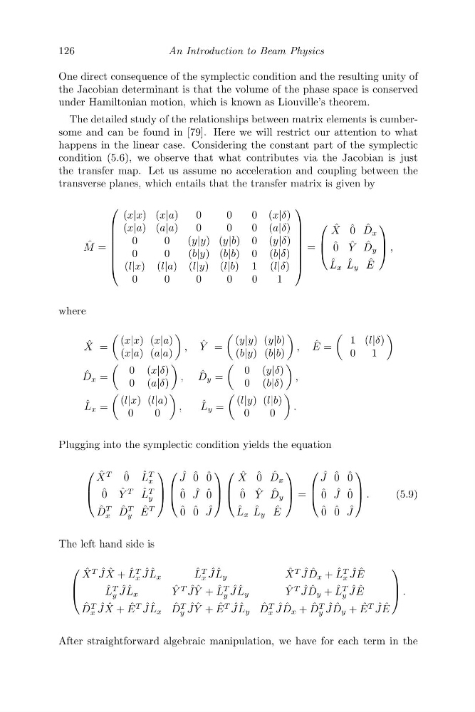
The detailed study of the relationships between matrix elements is cumbersome and can be found in [79]. Here we will restrict our attention to what
happens in the linear case. Considering the constant part of the symplectic
condition (5.6), we observe that what contributes via the Jacobian is just
the transfer map. Let us assume no acceleration and coupling between the
transverse planes, which entails that the transfer matrix is given by
ˆ
M =
⎛
⎜
⎜
⎜
⎜
⎜
⎜
⎝
(x|x) (x|a)
0
0
0 (x|δ)
(x|a) (a|a)
0
0
0 (a|δ)
0
0
(y|y) (y|b) 0 (y|δ)
0
0
(b|y) (b|b) 0 (b|δ)
(l|x) (l|a) (l|y) (l|b) 1 (l|δ)
0
0
0
0
0
1
⎞
⎟
⎟
⎟
⎟
⎟
⎟
⎠
=
⎛
⎜
⎝
ˆ
X ˆ 0 ˆ
D x
ˆ 0 ˆ
Y ˆ
D y
ˆ
L x ˆ
L y ˆ
E
⎞
⎟
⎠ ,
where
ˆ
X =
(x|x) (x|a)
(x|a) (a|a)
, ˆ
Y =
(y|y) (y|b)
(b|y) (b|b)
, ˆ
E =
1 (l|δ)
0
1
ˆ
D x =
0 (x|δ)
0 (a|δ)
,
ˆ
D y =
0 (y|δ)
0 (b|δ)
,
ˆ
L x =
(l|x) (l|a)
0
0
,
ˆ
L y =
(l|y) (l|b)
0
0
.
Plugging into the symplectic condition yields the equation
⎛
⎜
⎝
ˆ
X
T
ˆ 0 ˆ
L
T
x
ˆ 0 ˆ
Y
T ˆ
L
T
y
ˆ
D
T
x
ˆ
D
T
y
ˆ
E
T
⎞
⎟
⎠
⎛
⎜
⎝
ˆ
J ˆ 0 ˆ 0
ˆ 0 ˆ
J ˆ 0
ˆ 0 ˆ 0 ˆ
J
⎞
⎟
⎠
⎛
⎜
⎝
ˆ
X ˆ 0 ˆ
D x
ˆ 0 ˆ
Y ˆ
D y
ˆ
L x ˆ
L y ˆ
E
⎞
⎟
⎠ =
⎛
⎜
⎝
ˆ
J ˆ 0 ˆ 0
ˆ 0 ˆ
J ˆ 0
ˆ 0 ˆ 0 ˆ
J
⎞
⎟
⎠ .
(5.9)
The left hand side is
⎛
⎜
⎝
ˆ
X
T ˆ
J ˆ
X + ˆ
L
T
x
ˆ
J ˆ
L x
ˆ
L
T
x
ˆ
J ˆ
L y
ˆ
X
T ˆ
J ˆ
D x + ˆ
L
T
x
ˆ
J ˆ
E
ˆ
L
T
y
ˆ
J ˆ
L x
ˆ
Y
T ˆ
J ˆ
Y + ˆ
L
T
y
ˆ
J ˆ
L y
ˆ
Y
T ˆ
J ˆ
D y + ˆ
L
T
y
ˆ
J ˆ
E
ˆ
D
T
x
ˆ
J ˆ
X + ˆ
E
T ˆ
J ˆ
L x ˆ
D
T
y
ˆ
J ˆ
Y + ˆ
E
T ˆ
J ˆ
L y ˆ
D
T
x
ˆ
J ˆ
D x + ˆ
D
T
y
ˆ
J ˆ
D y + ˆ
E
T ˆ
J ˆ
E
⎞
⎟
⎠ .
After straightforward algebraic manipulation, we have for each term in the
An Introduction to Beam Physics
One direct consequence of the symplectic condition and the resulting unity of
the Jacobian determinant is that the volume of the phase space is conserved
under Hamiltonian motion, which is known as Liouville’s theorem.
The detailed study of the relationships between matrix elements is cumbersome and can be found in [79]. Here we will restrict our attention to what
happens in the linear case. Considering the constant part of the symplectic
condition (5.6), we observe that what contributes via the Jacobian is just
the transfer map. Let us assume no acceleration and coupling between the
transverse planes, which entails that the transfer matrix is given by
ˆ
M =
⎛
⎜
⎜
⎜
⎜
⎜
⎜
⎝
(x|x) (x|a)
0
0
0 (x|δ)
(x|a) (a|a)
0
0
0 (a|δ)
0
0
(y|y) (y|b) 0 (y|δ)
0
0
(b|y) (b|b) 0 (b|δ)
(l|x) (l|a) (l|y) (l|b) 1 (l|δ)
0
0
0
0
0
1
⎞
⎟
⎟
⎟
⎟
⎟
⎟
⎠
=
⎛
⎜
⎝
ˆ
X ˆ 0 ˆ
D x
ˆ 0 ˆ
Y ˆ
D y
ˆ
L x ˆ
L y ˆ
E
⎞
⎟
⎠ ,
where
ˆ
X =
(x|x) (x|a)
(x|a) (a|a)
, ˆ
Y =
(y|y) (y|b)
(b|y) (b|b)
, ˆ
E =
1 (l|δ)
0
1
ˆ
D x =
0 (x|δ)
0 (a|δ)
,
ˆ
D y =
0 (y|δ)
0 (b|δ)
,
ˆ
L x =
(l|x) (l|a)
0
0
,
ˆ
L y =
(l|y) (l|b)
0
0
.
Plugging into the symplectic condition yields the equation
⎛
⎜
⎝
ˆ
X
T
ˆ 0 ˆ
L
T
x
ˆ 0 ˆ
Y
T ˆ
L
T
y
ˆ
D
T
x
ˆ
D
T
y
ˆ
E
T
⎞
⎟
⎠
⎛
⎜
⎝
ˆ
J ˆ 0 ˆ 0
ˆ 0 ˆ
J ˆ 0
ˆ 0 ˆ 0 ˆ
J
⎞
⎟
⎠
⎛
⎜
⎝
ˆ
X ˆ 0 ˆ
D x
ˆ 0 ˆ
Y ˆ
D y
ˆ
L x ˆ
L y ˆ
E
⎞
⎟
⎠ =
⎛
⎜
⎝
ˆ
J ˆ 0 ˆ 0
ˆ 0 ˆ
J ˆ 0
ˆ 0 ˆ 0 ˆ
J
⎞
⎟
⎠ .
(5.9)
The left hand side is
⎛
⎜
⎝
ˆ
X
T ˆ
J ˆ
X + ˆ
L
T
x
ˆ
J ˆ
L x
ˆ
L
T
x
ˆ
J ˆ
L y
ˆ
X
T ˆ
J ˆ
D x + ˆ
L
T
x
ˆ
J ˆ
E
ˆ
L
T
y
ˆ
J ˆ
L x
ˆ
Y
T ˆ
J ˆ
Y + ˆ
L
T
y
ˆ
J ˆ
L y
ˆ
Y
T ˆ
J ˆ
D y + ˆ
L
T
y
ˆ
J ˆ
E
ˆ
D
T
x
ˆ
J ˆ
X + ˆ
E
T ˆ
J ˆ
L x ˆ
D
T
y
ˆ
J ˆ
Y + ˆ
E
T ˆ
J ˆ
L y ˆ
D
T
x
ˆ
J ˆ
D x + ˆ
D
T
y
ˆ
J ˆ
D y + ˆ
E
T ˆ
J ˆ
E
⎞
⎟
⎠ .
After straightforward algebraic manipulation, we have for each term in the