

The Linearization of the Equations of Motion
111
inverses, and integrated, resulting in substantially more terms than for the
previous order. Altogether, the effort increases extremely dramatically
with the order being considered, and for typical systems, it is practical only
to orders around five.
Computer codes that use the above procedure usually contain a library of
procedures that compute the aberrations for each particle optical element of
interest. The aberrations of combined systems is then determined from those
of the pieces with the help of a composition procedure. The Differential
Algebraic (DA) approach, as described in Chapter 5, allows the computation
of aberrations to any order in an elegant way without the need of explicit
formulas for aberrations.
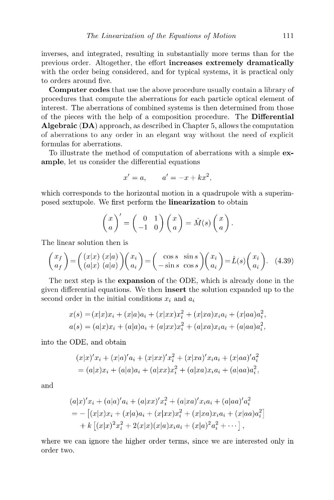
To illustrate the method of computation of aberrations with a simple example, let us consider the differential equations
x
= a,
a
= −x + kx
2 ,
which corresponds to the horizontal motion in a quadrupole with a superimposed sextupole. We first perform the linearization to obtain
x
a
=
0 1
−1 0
x
a
= ˆ
M (s)
x
a
.
The linear solution then is
x f
a f
=
(x|x) (x|a)
(a|x) (a|a)
x i
a i
=
cos s sin s
− sin s cos s
x i
a i
= ˆ
L(s)
x i
a i
. (4.39)
The next step is the expansion of the ODE, which is already done in the
given differential equations. We then insert the solution expanded up to the
second order in the initial conditions x i and a i
x(s) =(x|x)x i + (x|a)a i + (x|xx)x
2
i + (x|xa)x i a i + (x|aa)a
2
i ,
a(s) = (a|x)x i + (a|a)a i + (a|xx)x
2
i + (a|xa)x i a i + (a|aa)a
2
i ,
into the ODE, and obtain
(x|x)
x i + (x|a)
a i + (x|xx)
x
2
i + (x|xa)
x i a i + (x|aa)
a
2
i
= (a|x)x i + (a|a)a i + (a|xx)x
2
i + (a|xa)x i a i + (a|aa)a
2
i ,
and
(a|x)
x i + (a|a)
a i + (a|xx)
x
2
i + (a|xa)
x i a i + (a|aa)
a
2
i
= −
(x|x)x i + (x|a)a i + (x|xx)x
2
i + (x|xa)x i a i + (x|aa)a
2
i
+ k
(x|x)
2 x
2
i + 2(x|x)(x|a)x i a i + (x|a)
2 a
2
i + · · ·
,
where we can ignore the higher order terms, since we are interested only in
order two.
111
inverses, and integrated, resulting in substantially more terms than for the
previous order. Altogether, the effort increases extremely dramatically
with the order being considered, and for typical systems, it is practical only
to orders around five.
Computer codes that use the above procedure usually contain a library of
procedures that compute the aberrations for each particle optical element of
interest. The aberrations of combined systems is then determined from those
of the pieces with the help of a composition procedure. The Differential
Algebraic (DA) approach, as described in Chapter 5, allows the computation
of aberrations to any order in an elegant way without the need of explicit
formulas for aberrations.
To illustrate the method of computation of aberrations with a simple example, let us consider the differential equations
x
= a,
a
= −x + kx
2 ,
which corresponds to the horizontal motion in a quadrupole with a superimposed sextupole. We first perform the linearization to obtain
x
a
=
0 1
−1 0
x
a
= ˆ
M (s)
x
a
.
The linear solution then is
x f
a f
=
(x|x) (x|a)
(a|x) (a|a)
x i
a i
=
cos s sin s
− sin s cos s
x i
a i
= ˆ
L(s)
x i
a i
. (4.39)
The next step is the expansion of the ODE, which is already done in the
given differential equations. We then insert the solution expanded up to the
second order in the initial conditions x i and a i
x(s) =(x|x)x i + (x|a)a i + (x|xx)x
2
i + (x|xa)x i a i + (x|aa)a
2
i ,
a(s) = (a|x)x i + (a|a)a i + (a|xx)x
2
i + (a|xa)x i a i + (a|aa)a
2
i ,
into the ODE, and obtain
(x|x)
x i + (x|a)
a i + (x|xx)
x
2
i + (x|xa)
x i a i + (x|aa)
a
2
i
= (a|x)x i + (a|a)a i + (a|xx)x
2
i + (a|xa)x i a i + (a|aa)a
2
i ,
and
(a|x)
x i + (a|a)
a i + (a|xx)
x
2
i + (a|xa)
x i a i + (a|aa)
a
2
i
= −
(x|x)x i + (x|a)a i + (x|xx)x
2
i + (x|xa)x i a i + (x|aa)a
2
i
+ k
(x|x)
2 x
2
i + 2(x|x)(x|a)x i a i + (x|a)
2 a
2
i + · · ·
,
where we can ignore the higher order terms, since we are interested only in
order two.