

The Linearization of the Equations of Motion
109
the special case that ˆ
M is piecewise constant, then for every such piece,
one can try the ansatz l k = v k · exp(ω k s), which leads to the condition
ω k v k exp(ω k s) = ˆ
M · v k exp(ω k s),
an eigenvector problem. If ˆ
M has n distinct eigenvalues, we are done, and
depending on whether ω k is real or complex, the solutions can also be expressed in terms of sin, cos or sinh, cosh . In case of multiple eigenvalues,
often solutions of the form s · sin, etc., can be found.
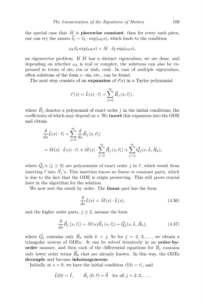
The next step consists of an expansion of r(s) in a Taylor polynomial
r (s) = ˆ
L(s) · r i +
∞
j=2
R j (s, , r i ) ,
where
R j denotes a polynomial of exact order j in the initial conditions, the
coefficients of which may depend on s. We insert this expansion into the ODE
and obtain
d
ds
ˆ
L(s) · r i +
∞
j=2
d
ds
R j (s, , r i )
= ˆ
M (s) · ˆ
L(s) · r i + ˆ
M (s) ·
∞
j=2
R j (s, , r i ) +
∞
j=2
Q j (s, ˆ
L,
R k ),
where
Q j ’s (j ≥ 2) are polynomials of exact order j in r, which result from
inserting r into
N j ’s. This insertion leaves no linear or constant parts, which
is due to the fact that the ODE is origin preserving. This will prove crucial
later in the algorithm for the solution.
We now sort the result by order. The linear part has the form
d
ds
ˆ
L(s) = ˆ
M (s) · ˆ
L(s),
(4.36)
and the higher order parts, j ≥ 2, assume the form
d
ds
R j (s, , r i ) = ˆ
M (s)
R j (s, , r i ) +
Q j (s, ˆ
L,
R k ),
(4.37)
where
Q j contains only
R k with k < j. So for j = 2, 3, . . . , we obtain a
triangular system of ODEs. It can be solved iteratively in an order-byorder manner, and then each of the differential equations for
R j contains
only lower order terms
R k that are already known. In this way, the ODEs
decouple and become inhomogeneous.
Initially at s = 0, we have the initial condition r(0) = r i , and
ˆ
L(0) = ˆ
I,
R j (0, , r) = 0 for all j = 2, 3, . . . .
109
the special case that ˆ
M is piecewise constant, then for every such piece,
one can try the ansatz l k = v k · exp(ω k s), which leads to the condition
ω k v k exp(ω k s) = ˆ
M · v k exp(ω k s),
an eigenvector problem. If ˆ
M has n distinct eigenvalues, we are done, and
depending on whether ω k is real or complex, the solutions can also be expressed in terms of sin, cos or sinh, cosh . In case of multiple eigenvalues,
often solutions of the form s · sin, etc., can be found.
The next step consists of an expansion of r(s) in a Taylor polynomial
r (s) = ˆ
L(s) · r i +
∞
j=2
R j (s, , r i ) ,
where
R j denotes a polynomial of exact order j in the initial conditions, the
coefficients of which may depend on s. We insert this expansion into the ODE
and obtain
d
ds
ˆ
L(s) · r i +
∞
j=2
d
ds
R j (s, , r i )
= ˆ
M (s) · ˆ
L(s) · r i + ˆ
M (s) ·
∞
j=2
R j (s, , r i ) +
∞
j=2
Q j (s, ˆ
L,
R k ),
where
Q j ’s (j ≥ 2) are polynomials of exact order j in r, which result from
inserting r into
N j ’s. This insertion leaves no linear or constant parts, which
is due to the fact that the ODE is origin preserving. This will prove crucial
later in the algorithm for the solution.
We now sort the result by order. The linear part has the form
d
ds
ˆ
L(s) = ˆ
M (s) · ˆ
L(s),
(4.36)
and the higher order parts, j ≥ 2, assume the form
d
ds
R j (s, , r i ) = ˆ
M (s)
R j (s, , r i ) +
Q j (s, ˆ
L,
R k ),
(4.37)
where
Q j contains only
R k with k < j. So for j = 2, 3, . . . , we obtain a
triangular system of ODEs. It can be solved iteratively in an order-byorder manner, and then each of the differential equations for
R j contains
only lower order terms
R k that are already known. In this way, the ODEs
decouple and become inhomogeneous.
Initially at s = 0, we have the initial condition r(0) = r i , and
ˆ
L(0) = ˆ
I,
R j (0, , r) = 0 for all j = 2, 3, . . . .