

�
�
84
Analytical Heat Transfer
q s ″
0
t
T (x,t)
T (x,t)
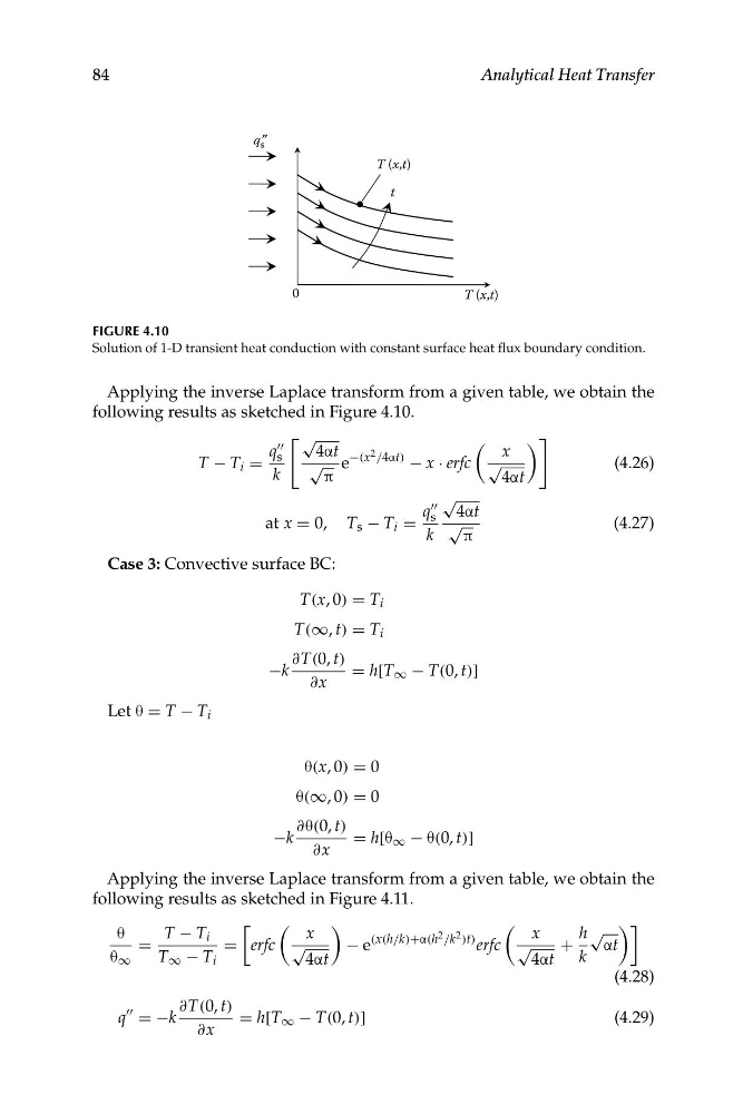
FIGURE 4.10
Solution of 1-D transient heat conduction with constant surface heat flux boundary condition.
Applying the inverse Laplace transform from a given table, we obtain the
following results as sketched in Figure 4.10.
� √
�
""
q
4αt
x
s
−(x
T − T i = k
√ π
e
2 /4αt)
− x · erfc √
(4.26)
4αt
√
""
q
4αt
s
at x = 0, T s − T i =
√
(4.27)
k
π
Case 3: Convective surface BC:
T(x, 0) = T i
T(∞, t) = T i
∂T(0, t)
−k
= h[T ∞ − T(0, t)]
∂x
Let θ = T − T i
θ(x, 0) = 0
θ(∞, 0) = 0
∂θ(0, t)
−k
= h[θ ∞ − θ(0, t)]
∂x
Applying the inverse Laplace transform from a given table, we obtain the
following results as sketched in Figure 4.11.
�
�
�
�
��
θ
T − T i
x
x
h √
=
= erfc √
− e
(x(h/k)+α(h 2 /k 2 )t) erfc √
+
αt
θ ∞
T ∞ − T i
4αt
4αt k
(4.28)
∂T(0, t)
""
q = −k
= h[T ∞ − T(0, t)]
(4.29)
∂x
�
84
Analytical Heat Transfer
q s ″
0
t
T (x,t)
T (x,t)
FIGURE 4.10
Solution of 1-D transient heat conduction with constant surface heat flux boundary condition.
Applying the inverse Laplace transform from a given table, we obtain the
following results as sketched in Figure 4.10.
� √
�
""
q
4αt
x
s
−(x
T − T i = k
√ π
e
2 /4αt)
− x · erfc √
(4.26)
4αt
√
""
q
4αt
s
at x = 0, T s − T i =
√
(4.27)
k
π
Case 3: Convective surface BC:
T(x, 0) = T i
T(∞, t) = T i
∂T(0, t)
−k
= h[T ∞ − T(0, t)]
∂x
Let θ = T − T i
θ(x, 0) = 0
θ(∞, 0) = 0
∂θ(0, t)
−k
= h[θ ∞ − θ(0, t)]
∂x
Applying the inverse Laplace transform from a given table, we obtain the
following results as sketched in Figure 4.11.
�
�
�
�
��
θ
T − T i
x
x
h √
=
= erfc √
− e
(x(h/k)+α(h 2 /k 2 )t) erfc √
+
αt
θ ∞
T ∞ − T i
4αt
4αt k
(4.28)
∂T(0, t)
""
q = −k
= h[T ∞ − T(0, t)]
(4.29)
∂x