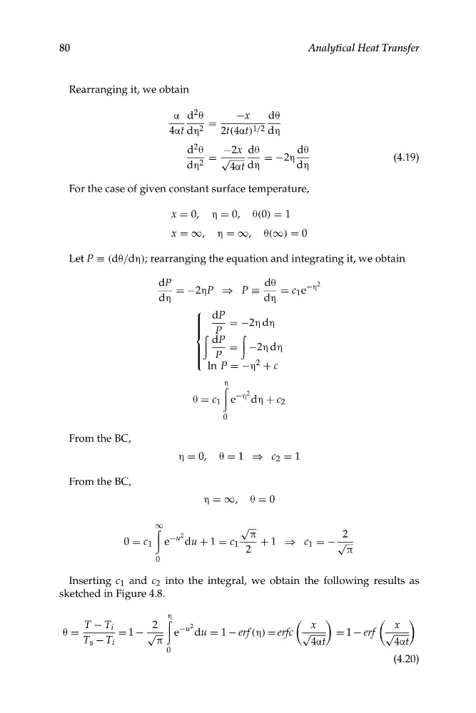
�
�
�
�
�
�
�
�
�
Rearranging it, we obtain
α d 2 θ
−x
dθ
=
4αt dη 2
2t(4αt) 1/2 dη
d 2 θ
−2x dθ
dθ
= √
= −2η
(4.19)
dη 2
4αt dη
dη
For the case of given constant surface temperature,
x = 0, η = 0, θ(0) = 1
x = ∞, η = ∞, θ(∞) = 0

Let P ≡ (dθ/dη); rearranging the equation and integrating it, we obtain

dP
dθ
η 2

= −2ηP ⇒ P ≡
= c 1 e
−
dη
dη
⎧ dP
⎪ ⎪
= −2η dη
⎪ ⎨ P
⎪ ⎪ ⎪
dP
P
= −2η dη
η 2 + c
⎩
ln P = −
η
θ = c 1 e
−η 2 dη + c 2
0
From the BC,
η = 0, θ = 1 ⇒ c 2 = 1
From the BC,
η = ∞, θ = 0
∞
√
2
π
2
−u
0 = c 1 e du + 1 = c 1
+ 1 ⇒ c 1 = −√
2
π
0
Inserting c 1 and c 2 into the integral, we obtain the following results as
sketched in Figure 4.8.
η
T − T i
2
e
2
x
x
−u
1 − √
du = 1 − erf (η) erfc √
1 − erf √
θ =
=
=
=
T s − T i
π
4αt
4αt
0
(4.20)
80
Analytical Heat Transfer